OLTP vs OLAP: Differences, Use Cases, and How They Work Together

Online transaction processing (OLTP) handles operational transactions such as order entry, payment recording, and stock-level checks. Online analytical processing (OLAP) supports complex queries that examine large data volumes for decision support. OLTP prioritizes reliable changes to operational records, and OLAP prioritizes analysis across many records.

These processing patterns can influence schema design, storage layout, indexing, concurrency control, and query execution. A database can provide capabilities associated with both OLTP and OLAP. Architects should evaluate each system against expected query patterns, transaction requirements, data freshness needs, and concurrency.

What Are the Main Differences Between OLAP And OLTP Databases?

The main difference is the work each system is designed to handle. OLTP typically processes concurrent operational transactions that create, retrieve, update, or delete a limited set of records. An OLAP database executes complex queries across larger datasets to support reporting, analysis, and decision-making. These priorities influence database design, optimization, and operational behavior. OLTP commonly emphasizes transaction integrity, selective access, and consistent outcomes under concurrent changes. OLAP commonly emphasizes scan efficiency, aggregation, and query throughput across analytical workloads.

Criterion	OLTP	OLAP
Primary purpose	Record and serve operational transactions	Analyze data for reporting and decision support
Typical operations	Short inserts, updates, deletes, and selective reads	Scans, joins, grouping, and aggregation
Records accessed	Usually one record or a limited subset	Commonly many records across tables or partitions
Workload pattern	Frequent, short transactions with defined consistency requirements	Read-intensive analytical queries; data can be loaded in scheduled batches or continuous streams
Concurrency	Many users or applications performing concurrent operational transactions	Multiple users or query streams executing analytical work
Schema design	Often normalized to support consistent inserts, updates, and deletes	Often dimensional or partially denormalized; normalized designs also exist
Physical storage	Row-oriented designs support selective lookups and whole-record access. Columnar or hybrid implementations can also serve operational workloads.	Column-oriented designs can reduce data reads when queries select a subset of columns. Row-oriented systems can also execute analytical queries.
Query optimization	Selective indexes and short access paths support targeted operations	Engines reduce data scanned and optimize joins, aggregations, and analytical query throughput
Data freshness	Usually reflects the current operational state after committed changes	May use scheduled loads, continuous ingestion, or current operational data
Common uses	Order entry, payment recording, delivery processing, order-status checks, and stock-level checks	Dashboards, reports, sales analysis, inventory analysis, trend analysis, and forecasting

Query and data access patterns

OLTP applications commonly issue predefined operations that target a limited set of records. Examples include entering orders, recording payments, checking order status, and monitoring stock levels. Matching indexes can give the database a short access path to relevant records.

OLAP queries commonly examine broader data ranges across multiple tables or partitions. They may scan many records, join tables, group values, and calculate aggregates. The amount of data read depends on filters, referenced columns, storage metadata, and physical design.

Some analytical systems like Exasol use an MPP database architecture to distribute scans, joins, and aggregations across multiple processing nodes. Performance still depends on data distribution, query design, and concurrent demand.

Schema and physical storage

OLTP systems often use normalized schemas to reduce redundancy and support consistent updates. Analytical systems often use dimensional or partially denormalized models to reduce join complexity in common queries. The choice between normalization and denormalization depends on query patterns, update behavior, and consistency requirements.

Logical schema and physical storage remain separate design choices. Row vs column storage models support different access patterns. Row-oriented storage can support targeted lookups and whole-record access. Column-oriented storage can reduce data reads when queries reference a limited subset of columns.

Transactions and concurrency

OLTP suitability requires examining isolation levels, locking granularity, update contention, and retry behavior. Database engines may use locks, multiversion concurrency control, or both to coordinate concurrent access. These mechanisms influence which operations can proceed while other transactions read or change data.

Analytical concurrency requires evaluating processor, memory, and storage demand across simultaneous queries. TPC-H measures throughput by running multiple query streams concurrently with a refresh stream. Production tests should represent expected queries, data distributions, arrival patterns, and concurrency.

These criteria describe common workload patterns, and implementations vary across products and configurations. Architects should test the complete database implementation with representative workloads across all relevant criteria.

OLTP and OLAP Query Examples

The following examples use a simplified order schema and illustrative SQL. Transaction-control syntax and error behavior vary by database engine and client. Query shape, records touched, write frequency, and concurrency determine the workload classification.

Recording an order

The first example inserts one order header and two line-item records inside a transaction. An application can commit the statements after validation or roll them back when an error occurs. Production order processing may also update inventory, enforce constraints, and apply application-specific business rules.

START TRANSACTION;

INSERT INTO orders (
    order_id,
    customer_id,
    order_date,
    status,
    sales_region
)
VALUES (10482, 7821, DATE '2025-03-14', 'PENDING', 'WEST');

INSERT INTO order_items (
    order_id,
    line_number,
    product_id,
    quantity,
    unit_price
)
VALUES
    (10482, 1, 991, 2, 49.95),
    (10482, 2, 447, 1, 129.00);

COMMIT;

This operation creates a limited group of related records. The transaction groups the order header and line items into one unit of work. Constraints, isolation settings, and application logic determine how the system handles conflicts and failures.

Analyzing order revenue

The second example calculates completed-order revenue by sales region for one reporting period.

SELECT
    o.sales_region,
    SUM(oi.quantity * oi.unit_price) AS revenue
FROM orders AS o
JOIN order_items AS oi
    ON o.order_id = oi.order_id
WHERE o.order_date >= DATE '2025-01-01'
  AND o.order_date < DATE '2026-01-01'
  AND o.status = 'COMPLETED'
GROUP BY o.sales_region
ORDER BY revenue DESC;

This query joins order headers with line items, filters completed orders, and aggregates revenue by sales region. A small result set can require the engine to process many qualifying input rows. The physical work depends on data volume, statistics, indexes, partitions, storage layout, and the selected execution plan.

The transactional operation changes a limited group of related records. The analytical query summarizes records across a reporting period and category. Actual suitability depends on concurrency, latency targets, isolation requirements, and measured workload behavior.

How OLTP and OLAP Work Together

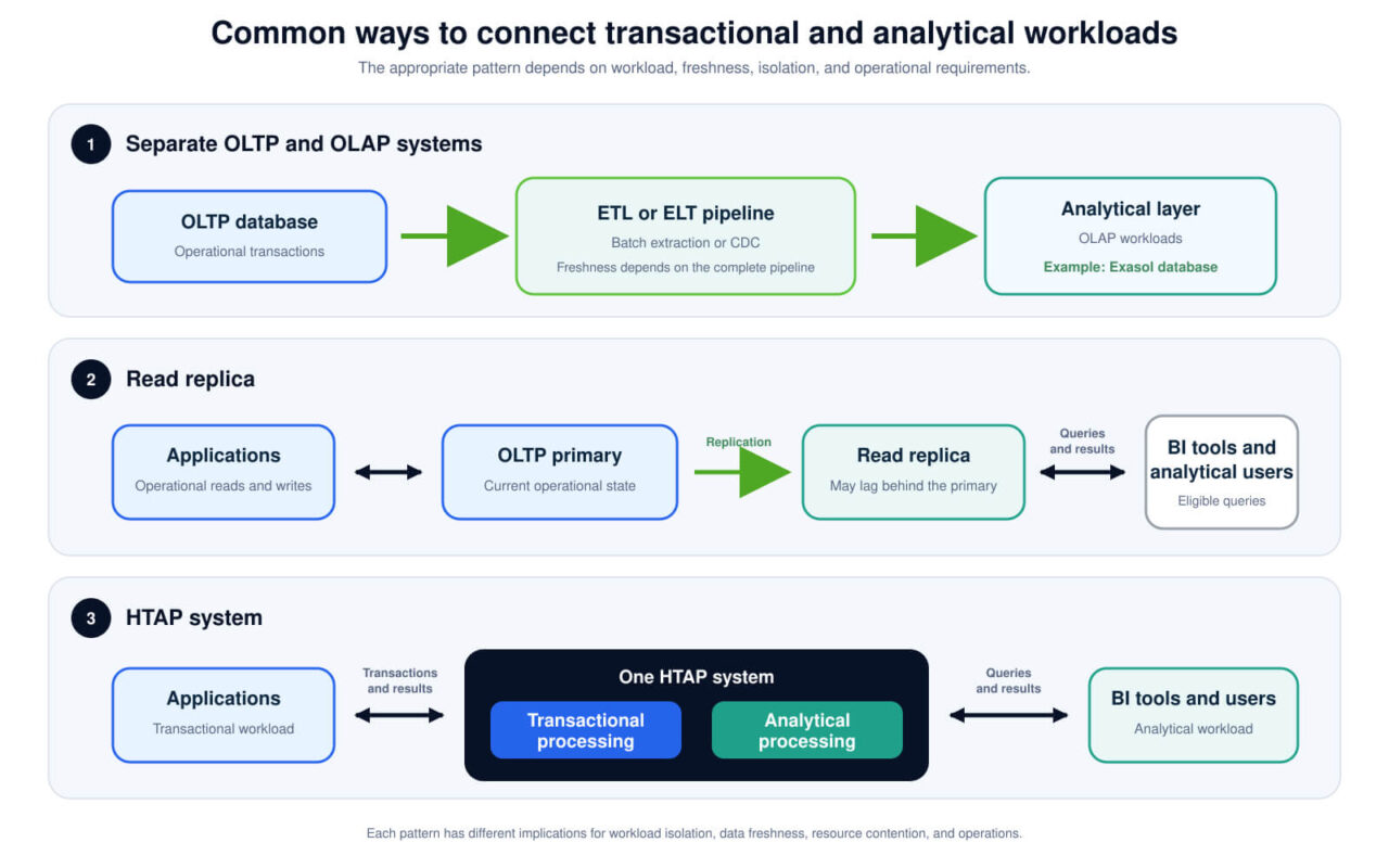
OLTP and OLAP commonly operate as parts of one data architecture. Operational systems record changes, and analytical systems consume copies or representations of the resulting data. The connection may use scheduled pipelines, continuous change streams, replicas, or a mixed-workload database design.

ETL, ELT, and change data capture

Extract, transform, and load (ETL) processes transform source data before loading it into an analytical target. Extract, load, and transform (ELT) processes load source data first and perform transformations in the target. Both patterns can populate a data warehouse from one or more operational systems.

The selected load schedule determines when new source data becomes available for analysis. Log-based change data capture (CDC) extracts persistent changes from a transaction log and streams them to downstream consumers. End-to-end freshness depends on capture, transport, transformation, target ingestion, and processing backlogs.

CDC recovery, delivery, and large-transaction behavior varies by source, connector, and target. Verify those behaviors in the documentation for the selected components. Recovery and delivery behavior should be verified for the selected source, connector, and target.

Read replicas and workload isolation

A read replica can serve eligible analytical queries using a copy of operational data. This moves query execution away from the primary system. Replica queries still consume processor, memory, and storage resources on the replica.

Replica data may lag behind the primary, producing different results for queries executed at the same time. Some implementations may delay or cancel replica queries when recovery conflicts with changes from the primary. Architects should evaluate acceptable lag, query duration, recovery behavior, and failover requirements.

A dedicated OLAP system separates analytical execution from the transaction database and allows independent physical design. It introduces another system to operate. If the design copies source data, it also requires data movement and an explicit freshness objective.

HTAP and mixed workloads

Hybrid transactional and analytical processing (HTAP) runs transactional and analytical workloads within one database system. Implementations may use separate access structures or storage representations within the same platform. Shared-platform designs can reduce external data movement and freshness delays for supported workloads.

Mixed workloads can still compete for processor time, memory, and storage input and output. Analytical structures maintained alongside transactional data can also add work to inserts, updates, and deletes. Resource management and physical design determine how much one workload affects another.

Evaluate transaction latency, analytical response time, ingestion, data freshness, and concurrency together. Tests should represent the expected query mix, transaction mix, data-change rate, and concurrent demand. The results may support a mixed-workload system, isolated replicas, or separate OLTP and OLAP systems.

Which Scenarios Are Best Suited for OLAP Versus OLTP?

Use OLTP for frequent operational transactions that create or change a small set of records. Use OLAP for analytical queries that scan, join, and aggregate broader datasets. An architecture can support both patterns when applications require operational processing and analysis. Treat these choices as starting points, then validate them against the workload and service objectives.

Scenario	Typical starting point	What to validate
Record orders, payments, or inventory changes	OLTP	Transaction guarantees, contention, throughput, and response time
Retrieve or update a current operational record	OLTP	Access paths, consistency, and behavior under concurrent demand
Run dashboards or reports over historical data	OLAP	Query response, throughput, data volume, and freshness
Run ad hoc joins and aggregations across broad periods	OLAP	Query mix, scan volume, aggregation behavior, and concurrency
Analyze near-current data from one operational source	Mixed workload, readable secondary, or dedicated OLAP system	Transaction overhead, resource contention, and acceptable data latency
Combine multiple sources or protect transaction service objectives	Separate OLTP and OLAP systems	Data movement, analytical freshness, and operational responsibility

Choose OLTP for operational transactions

Choose OLTP when an application must create or update operational state through frequent, short transactions. Common examples include order entry, payment recording, inventory changes, order-status checks, and stock-level checks. Evaluate atomicity, consistency, isolation, durability, contention, throughput, and response time under concurrent writes.

OLTP also supports targeted reads tied to operational workflows, such as retrieving a current order or account record. Evaluate transaction guarantees, access paths, storage, and contention behavior together. Test these characteristics under representative concurrent demand.

Choose OLAP for analytical queries

Choose OLAP when users need to scan, join, filter, and aggregate data across many records. Common scenarios include business intelligence dashboards, financial reporting, sales analysis, inventory analysis, trend analysis, and forecasting.

An OLAP database fits workloads that summarize data across time periods, categories, or business entities. For high-concurrency BI, measure query response and throughput with representative data and concurrent query streams.

Some analytical environments use an OLAP cube to organize measures across dimensions such as time, product, and region.

Use separate systems when workloads compete

Dedicated OLTP and OLAP systems can isolate transaction processing from analytical resource demand. This architecture introduces an additional system to operate. When data is copied into the analytical system, it also introduces data movement and potential latency between source changes and analytical availability.

A mixed-workload system can fit when one platform meets both service objectives under representative load. Test transaction response time and analytical throughput concurrently. Use workload isolation or separate systems when measured contention prevents either workload from meeting its requirements.

Where The Exasol Database Fits

The Exasol database is an in-memory, columnar analytics database. As an MPP database, it distributes analytical workloads across cluster nodes for near-real-time analytics, data warehousing, and AI /ML workloads. In a separated OLTP and OLAP architecture, it fits the analytical layer. The operational database handles application transactions, and the Exasol database serves reporting, dashboards, analytical SQL, and AI model execution.

Its massively parallel processing (MPP) shared-nothing architecture distributes data and query execution across cluster nodes. Each node processes its local data, and the database returns a combined result to the client. Response time and throughput require representative testing.

Two documented integration methods are relevant to a separated architecture. JDBC IMPORT loads data from another database into the Exasol database. Virtual schemas expose external data as virtual tables that can be queried alongside persistent Exasol tables. Choose between persisted loads and virtual access based on freshness, source-system load, data volume, and end-to-end query requirements. Validate the selected pattern with representative data and concurrent queries.

There are three AI model paths: in-database models, self-hosted or sovereign cloud models, and hosted cloud APIs. In-database models run as SQL-callable user-defined functions and keep data in the Exasol database. Self-hosted and sovereign cloud models can keep data within an organization-controlled environment. Hosted cloud APIs send data outside the Exasol environment. Architects should select a path according to model capability, data residency, governance, performance, and operating requirements.

The Exasol MCP Server connects compatible AI assistants to database metadata, schemas, and SQL execution. Database-user permissions determine query access. Exasol recommends a dedicated least-privilege account for AI assistant access. OLTP and OLAP describe workload priorities, not fixed product categories. Choose OLTP for frequent operational transactions and OLAP for broad analytical queries, then test concurrency, freshness, and latency with representative workloads. In architectures that separate the two, the Exasol database can serve the analytical layer for reporting, dashboards, analytical SQL, and supported AI/ML workloads.