

Seeing Your Processes for What They Really Are – Not What You Think They Are

How Process Mining Demonstrator Turns Business Event Data into Clarity
There is a well-known gap in almost every organization. On one side sits the process model – the flowchart that was designed in a workshop, approved by management, documented in the quality handbook, and presented in onboarding training. On the other side sits reality: the day-to-day stream of actual events logged by the systems that support the work. Between those two things is usually a significant distance.
Most of the time, that distance goes unmeasured. Individual team members have a feel for it. Experienced managers know which steps are routinely skipped, which workarounds have quietly become standard practice, which parts of the process slow down without warning when volumes increase. But this knowledge is fragmented, informal, and invisible to the organization as a whole.
The consequences are real. Improvement projects are designed to fix problems described from memory rather than measured with data. Compliance checks compare documentation to documentation rather than documentation to behavior. Automation initiatives are built on the assumption that the process is what it says it is, only to discover after go-live that half the variants were never modeled.
Process mining is the discipline of closing that gap. It takes the event logs your business systems already produce and uses them to reconstruct how work actually flows. Not how it was designed to flow. How it does flow.
Process Mining Demonstrator is a native Mac application that brings process mining capabilities to analysts, managers, and improvement practitioners – without requiring a data science background or a dedicated analytics team. The application is for demonstration or educational purposes only. I am using the application to bring the principle of Process Mining as an additional use case to customers and partners.
The Three Questions Every Business Needs to Answer
Before describing the application’s features, it is worth being precise about the problem structure it is designed for. There are three distinct levels of understanding that organizations need when something in a business process is not performing as expected. They are often confused with each other, and using the wrong tool at the wrong level is one of the most common reasons process improvement work stalls.
Level 1: What?
The first level is detection. Something is wrong, or something has changed. Dashboards exist for this purpose. A set of KPIs displayed with a traffic-light system – green meaning acceptable, amber meaning watch, red meaning act – tells you at a glance what is happening across your operations. Cycle time is red. SLA compliance has dropped to amber. Customer satisfaction has moved from green to amber over the past three weeks.
This level is well served by most business intelligence tools. It is important and necessary, but it has a firm limit: it tells you that something is wrong. It does not tell you why.
Level 2: Why?
The second level is diagnosis. When you see a red KPI on a dashboard, your natural response is to ask: what is going on inside this process that is producing this result? This is the level at which the Process Mining Demonstrator operates.
The data that answers “why” comes from your transactional systems – your ERP, your CRM, your ticketing platform, your order management system. These systems record what happened in business terms: an order was placed, a claim was submitted, a ticket was opened, a payment was processed. They record the business-level steps and when they occurred. Aggregated and analyzed as a process, this data reveals which routes cases are taking, where delays are accumulating, which segments are underperforming, and how the current behavior compares to the intended design.
The drill-down from dashboard to process map is the journey from what to why. When the SLA dashboard turns red, opening the Process Mining Demonstrator and examining the process map for the affected period and segment will show you where in the process time is being lost. The answer is almost never “everywhere” – it is almost always specific to one or two transitions, one or two routes, one or two segments. Making that specificity visible is the purpose of process mining.
Level 3: How?
The third level is the deepest and, in many organizations, the least explored. Once you know why a problem is occurring at the business process level, a further question often remains: how did this actually happen in the systems? At the technical level, step by step, what sequence of events produced this outcome?
Transactional data cannot answer this question. It records business events – coarse-grained, intended, user-initiated milestones. It does not record the system-level activity between those milestones: the API calls made, the queues traversed, the service that timed out and retried, the database transaction that locked and waited, the automated rule that fired unexpectedly.
Answering “how” requires a different kind of source data: system log files.
Modern business applications generate extensive logs – application servers, integration middleware, workflow engines, API gateways, databases. Each of these writes events at a technical level, with high precision. The challenge is that these logs come from different systems, use different formats, and speak different vocabularies. They are almost never analyzed together. Connecting the technical trail across multiple systems to a single business-level case is the work that unlocks the “how.”
The Data Structure That Makes Process Mining Possible
Whether you are working at the “why” level with transactional data or the “how” level with system logs, analysis becomes possible only once the raw data is organized into a single, consistent structure. This structure is simple – deliberately so. It has three required columns and a small number of optional ones.
The Required Core
| Column | Description |
|---|---|
CASE_ID | A unique identifier for the journey – the thread connecting all events belonging to one case. An order number, a claim reference, a ticket ID, a session token, a transaction ID. |
| Column | Description |
|---|---|
STEP | The name of the activity or event that occurred. “Order received”, “Credit check passed” for transactional data. “API call initiated”, “Timeout error”, “Retry attempt 2” for log data. |
TIMESTAMP | When the event occurred – date and time for business processes, milliseconds for technical event logs. |
These three columns are enough to reconstruct a process. Every journey is a sequence of (CASE_ID, STEP, TIMESTAMP) triples, ordered by time. Aggregate enough journeys and the process emerges.
The Optional Enrichment Columns
| Column | Description |
|---|---|
META_1 | A first business dimension – customer segment, product category, region, priority class, or any attribute that might explain variation. |
META_2 | A second business dimension – team, system version, channel, contract type, or similar. |
META_3 | A third business dimension for a further cut of the data. |
SCORE | A numeric outcome indicator – a customer satisfaction score, a quality control result, a compliance rating. |
From Logs to This Structure
The transformation from raw log files to this structure is the integration step that makes the “how” level of analysis accessible. A log entry from a middleware server might look like:
2026-03-14T09:23:11.442Z [INFO] TxID=ORD-884421 svc=payment-gateway
event=AUTHORISATION_REQUESTED latency_ms=234
Mapped to the event structure, this becomes:
CASE_ID | STEP | TIMESTAMP |
| ORD-884421 | AUTHORISATION_REQUESTED | 2026-03-14 09:23:11 |
The same order ID also appears in the transactional system as a business-level case. Once log events are mapped to the same structure and the same case identifier, the technical trail and the business trail can be analyzed together – or independently – using exactly the same process mining tools.
This is what makes the data structure powerful despite its simplicity. It imposes no constraints on what a “step” means. It works equally well for a business process spanning days and for a technical transaction spanning milliseconds. The analytics are the same. The questions are different.
How the Traffic Light Becomes a Map
In practice, the journey from dashboard to process map to system log analysis follows a natural investigation arc.
A compliance dashboard shows that SLA performance for a particular claims category has dropped from 94% to 79% over the last two months. That is the amber light – the what.
An analyst opens Process Mining Demonstrator and filters the process map to that claims category, for the last two months, for cases that breached SLA. The map immediately shows that breaching cases overwhelmingly take a route through a manual reassessment step that does not appear in compliant cases. The average time for a case to move from submission to re-assessment is eleven days, compared with an average of 1 day for all other transitions. The why is now visible: a specific step, on a specific route, is absorbing almost all of the excess time.
But why is the re-assessment step slow? That question cannot be answered from transactional data. The next step is to pull the system log data from the workflow engine that manages the re-assessment queue, map it to the event structure with the same claim IDs, and analyze it as a separate process project. The technical process map shows that reassessment tasks are being correctly assigned but then left unactioned – not because staff is absent, but because a notification service that triggers email alerts when tasks arrive is silently failing. The how is a technical fault invisible in any business-level report.
Three levels of data. Three levels of question. One analytical approach, applied consistently.
The Process Map: Seeing the Flow
The centerpiece of Process Mining Demonstrator is the Process Map – a flow diagram drawn by data, not by a workshop facilitator.
Each box represents a step that appears in the event log. Each arrow represents a transition that was observed in the data. The width of the arrow reflects how often that route is taken. A thick line between two steps means most cases travel that way. A thin line means only a handful do.
This alone is often revelatory:
- Steps in the data but not in the model – activities happening that were never documented
- Steps in the model but almost never in the data – approved steps that have been quietly abandoned
- Loops and rework cycles – cases traveling backward through the process before progressing
- Shortcuts – cases skipping intermediate steps, sometimes legitimately, sometimes not
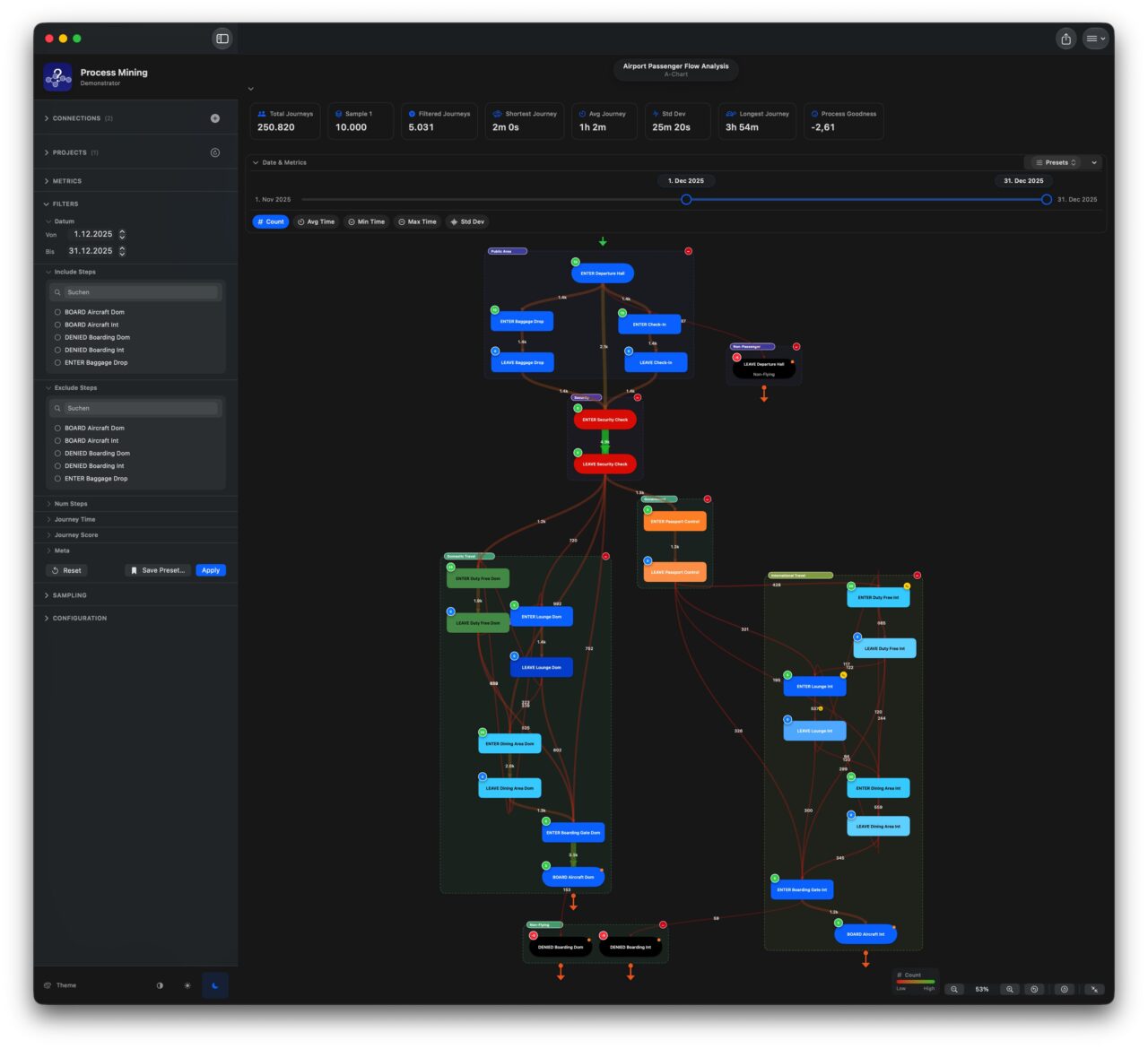
You can color the connecting arrows by frequency, average duration, maximum wait time, or variability. Standard deviation of transition time is often the most informative: a step that sometimes takes two hours and sometimes takes three weeks points to an unmanaged dependency, an informal escalation path, or a handover that works reliably only when certain people are available.
Filtering: Getting to the Right Question
A process map of all your data, all at once, shows what is typical. Most business questions are about specific subsets.
The sidebar gives you filters that narrow the data to exactly the population you are asking about. All maps, charts, and statistics update instantly as you adjust filters.
Date range answers the before-and-after questions that follow every change, every peak period, every incident.
Metadata dimensions answer the segment questions: same nominal process, different customer types, different regions, different teams. The META_1, META_2, META_3 columns in the event structure directly power these filters.
Journey characteristics let you focus on the outliers: the longest cases, the most complex, the ones that exceeded the SLA, the ones that scored below threshold. The populations that most need attention are rarely the typical ones.
Saved filter presets give teams a shared vocabulary of standard analytical views, defined once and reused consistently.
Happy Path: Measuring Conformance
Knowing what the process does is valuable. Knowing how far it deviates from what it should do is actionable.
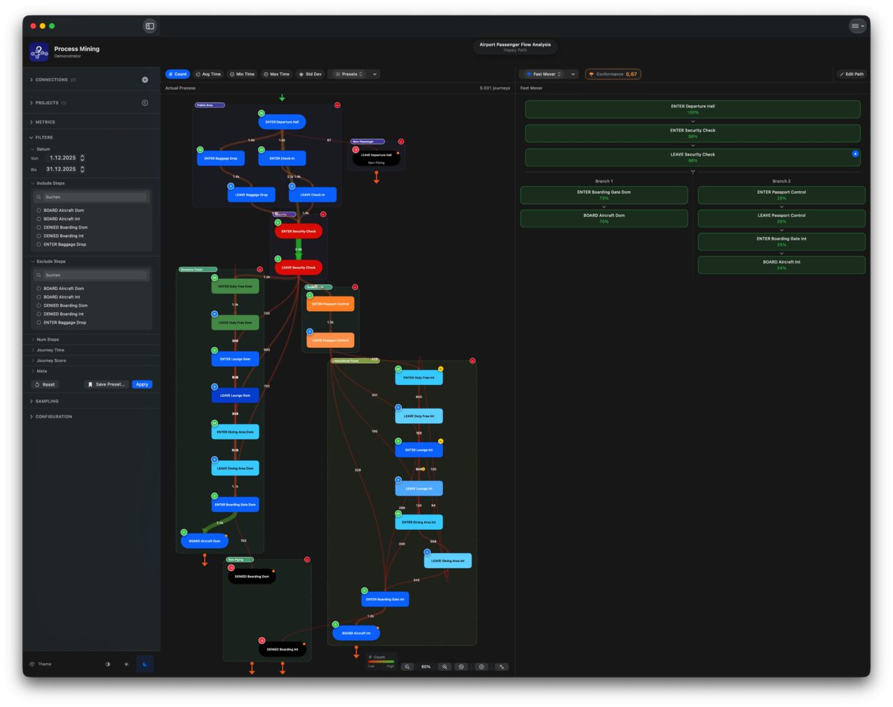
The Happy Path feature lets you define the ideal sequence of steps – the path that is efficient, compliant, and produces the best outcome. Optional branches accommodate known legitimate variants. The app then measures, across all journeys in the current filtered view, how often reality matches that definition and produces a conformance score.
Use Case: Compliance Monitoring
A financial services firm runs a loan approval process. Regulations require that every application is checked by a credit risk assessor before any approval decision is made. The happy path includes that step. The conformance score tells the compliance team, at any point in time and for any slice of the portfolio, what percentage of applications actually received that check. If the score drops, an investigation is warranted.
Use Case: Post-Change Validation
An IT team has redesigned the incident resolution process, eliminating a redundant peer review step and adding a mandatory root cause documentation step before closure. They define the new happy path, then filter the data to the weeks since the change went live. A conformance score of 72% indicates that 28% of incidents are still being closed without the root cause step – old habits persist. The map shows which teams are responsible for most of the non-conforming cases.
Use Case: Process Quality Tracking Over Time
A customer onboarding team wants to track how well their process is being followed as volumes grow and new staff join. They define the happy path, save the filter preset, and check the conformance score monthly. When it begins declining, they know to investigate before the problem becomes embedded. The conformance score feeds directly back into the dashboard layer as a KPI – one more traffic light, this time grounded in observed behavior rather than self-reported compliance.
A/B Comparison: Measuring Change and Difference
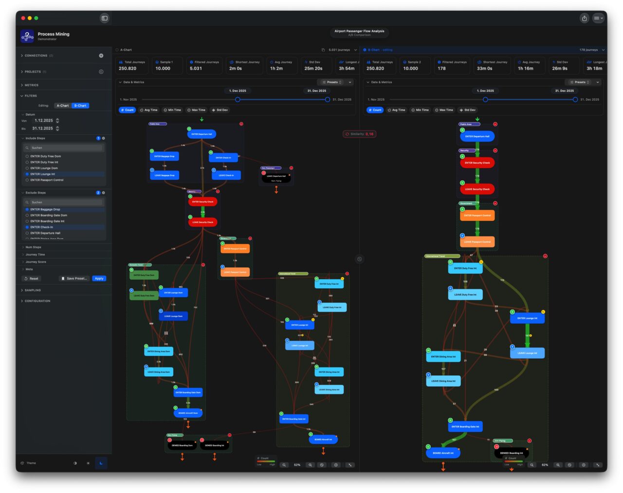
Some of the most valuable process questions are comparative. The A/B view places two process snapshots side by side – different time periods, different segments, or different sample sets from the same data.
A similarity score summarises the structural relationship between the two processes. Near 100% means essentially the same behavior. Near 0% means fundamentally different processes. Most real comparisons sit somewhere in the middle, and the score provides an objective measure to track.
Use Case: Before and After a System Change
An operations team migrates their order management system. Six weeks later, they open the A/B view with the six months before the migration on side A and the six weeks after on side B. The similarity score is 67%. The maps show that a rework loop – orders being returned for manual correction after an automated check – has almost disappeared on side B. The new system is catching the issue upstream. That finding goes into the post-implementation review as a measurable, data-backed benefit.
Use Case: Segment Comparison
A claims manager suspects that claims from one regional office take significantly longer than those from other regional offices. Side A is filtered to that region, side B to all others. The A/B view immediately confirms the suspicion: the map on side A shows a large loop that appears only faintly on side B, indicating a manual re-keying step that the regional office’s legacy system still requires. The finding is specific enough to act on.
Use Case: Fast Cases versus Slow Cases
A process improvement team defines “fast cases” as journeys that complete in under three days and “slow cases” as those that take more than two weeks. Side A shows fast cases, side B shows slow cases. The structural differences in the two maps tell the team exactly what characterizes each population. The slow cases consistently have a specific approval step that fast cases avoid, and they are concentrated in one product category. The root cause is visible and addressable.
Statistics: Going Deeper into the Numbers
The Statistics view provides the quantitative underpinning of the visual map.
A journey duration histogram shows how completion times are distributed. A narrow peak means a consistent process. A wide spread means high variability. A bimodal distribution – two distinct peaks – suggests two populations with fundamentally different behavior sharing a single process name, which often means they should be managed separately.
A journey path table ranks every distinct route taken through the process by frequency. The answer to “how many different actual sequences are our cases following?” is almost always much higher than anyone expects. Making it visible is the starting point for deciding which variants are acceptable and which represent problems.
A transition heatmap shows every step pair and how frequently cases moved directly from one to the other. Unexpected dark cells – transitions that happen constantly despite no explicit route in the process design – are among the most reliable indicators that a workaround has become standard practice.
A journey volume timeline shows how case volumes vary across the period covered by the data. A spike that coincides with a drop in conformance or an increase in average duration is a causal hypothesis worth investigating.
Sampling: Working Responsibly with Large Datasets
Real business event logs are large. The Sampling feature lets you create up to three named representative subsets – smaller populations that load and respond quickly but carry the statistical properties of the full dataset.
Random sampling gives a statistically fair cross-section of all journeys.
Temporal stratified sampling ensures all time periods are represented proportionally – essential when process volumes vary significantly across seasons or business cycles.
Path diversity sampling deliberately includes cases from across the full range of routes, including the rare ones. A route taken by 2% of cases may be statistically rare but operationally critical – particularly if those 2% represent your highest-value customers or highest-risk transactions.
Simulation: Testing Ideas Before They Become Reality
Every significant process change carries risk. Remove a step, and you might eliminate a bottleneck – or you might remove a control that was preventing errors you never noticed. Add a mandatory checkpoint, and you might improve compliance – or you might create a new queue that slows down every case. The honest answer to “what will happen if we change this?” is almost always: we don’t know, but we can make it an informed question.
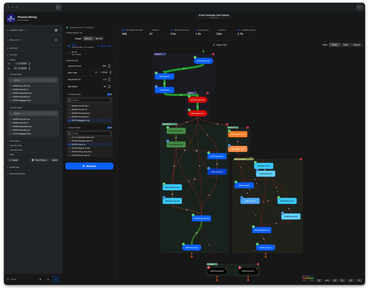
The Simulation feature gives you a structured way to answer that question before committing to any change. It learns the statistical behavior of your process from the real data – how often each route is taken, how long each transition typically takes, how much that timing varies – and uses that model to generate realistic synthetic journeys that behave like plausible future cases. Every tool in the application works identically on simulated data as on historical data. And because the journeys are synthetic, there is zero operational risk: no real cases are touched, no live system is affected, nothing is deployed.
Why Simulation Is Not Just Guesswork
The critical distinction between simulation and estimation is that simulation is grounded in your actual data rather than assumptions. Two statistical models are extracted directly from the real event log before a single synthetic journey is produced.
The routing model maps the probability of every transition in the process as it actually occurred. If the real data show that, after “Credit Check,” a case moves to “Approval” 78% of the time and to “Manual Review” 22% of the time, the model captures exactly that ratio. This is done for every step in the process, forming a complete probability map – a picture of how likely it is, from any point in the workflow, that a case will take each available route forward. This approach, known as a Markov chain, ensures the simulation reflects the actual distribution of routes in your process, rather than a simplified flowchart.
The timing model captures how long each transition takes, including the natural variability. Most business process durations follow a characteristic shape: the majority of cases are fast, clustered around the typical time, but a tail of slower cases extends outward – a few take twice as long, and occasionally one takes dramatically longer. The simulation fits a lognormal distribution to each transition individually, matching both the average pace and the spread. This means simulated journeys include the same natural variation seen in real cases – they are not uniformly average, but realistically mixed.
New cases arrive following a Poisson process – the standard model for random arrivals used throughout operations research and service design. You specify the average interval between arrivals; the engine distributes them to produce natural clustering and gaps rather than perfectly even spacing, matching the pattern of real business-case arrivals.
What You Can Control
Beyond the statistical model itself, three parameters shape each simulation run:
Journey count and time window – how many synthetic cases to generate, and when the simulation starts. Running a larger count reduces statistical noise; running it at a future date lets you assess a proposed change in a future context.
Excluding steps removes them from the model before any journeys are generated. Every transition leading to or from the excluded step is removed, and the model is then re-evaluated for reachability – any step that only received work from the excluded step is pruned as well. The result is a structurally clean model of the process as it would exist if those steps genuinely did not exist. This is how you simulate removing a bottleneck, eliminating a legacy approval, or consolidating two steps into one.
Requiring steps serves as a post-generation filter: only journeys that passed through all required steps are kept. This simulates the effect of making a step mandatory – useful for modeling a new compliance checkpoint, a mandatory quality review, or any step the redesigned process insists must occur.
Two Named Scenarios: Sim-A and Sim-B
This is where simulation moves from analysis to decision support.
Each simulation run can be stored in one of two named slots: Sim-A and Sim-B. Think of them as labeled scenarios – “Option A” and “Option B” of a proposed process change. A segmented control in the simulation panel lets you choose which slot each run targets before you press Simulate. Once stored, each slot shows its status: the journey count, the number of distinct variants, and the KPIs from that run.
Storing two scenarios opens the full comparison toolkit – the same A/B infrastructure used for real data now works equally on simulation results and on any combination of the two.
Comparing Scenarios with the Full A/B Toolkit
From the simulation panel, a single button loads a scenario directly into the A/B comparison view. Both simulation slots and all real data sample sets are available as sources for each side of the A/B view simultaneously, which means you can construct any of these comparisons:
| Side A | Side B | Question answered |
|---|---|---|
| Sim-A | Sim-B | Which of these two redesign options produces the better process? |
| Original data | Sim-A | How different would the process be after Option A? How big is the impact? |
| Original data | Sim-B | What does Option B look like against the current baseline? |
| Sim-A | Sim-B | If both options achieve similar conformance, which runs faster? |
| Sample 1 (pre-change) | Sim-A | Will Option A return us closer to our historical baseline? |
The A/B view provides a similarity score between the two sides – a single number expressing how structurally alike the two processes are. A high score between Sim-A and Sim-B indicates that the two proposed options exhibit nearly the same process behavior. A low score means they diverge substantially, and the side-by-side process maps show exactly where. This is the difference between walking into a decision meeting with an opinion and walking in with a measurement.
You can also check simulated journeys against a happy path – the defined ideal process. The conformance score for Sim-A tells you what proportion of cases in that scenario would follow the intended route if the change were implemented. If Option A has a conformance score of 62% and Option B has 89%, the choice is data-backed rather than debated.
Business Use Cases
Pre-change impact assessment: Before removing a manual quality check from a claims-handling process, run Sim-A without that step and compare it to the original data in the A/B view. The similarity score and process maps show how much the flow would change. The duration KPIs indicate whether the expected cycle-time reduction is meaningful or marginal.
Choosing between two redesign options – A process redesign team has two proposals: Option A removes an intermediate approval step; Option B replaces it with an automated rule. Store each as Sim-A and Sim-B. Compare them in A/B. The option with the better combination of conformance score, average cycle time, and process similarity to the intended design has the evidence to proceed.
Compliance pre-testing – Before rolling out a new mandatory documentation step required by a regulatory change, simulate the new process with that step required. Check the conformance score against the existing happy path. If only 60% of simulated cases naturally flow through the new step, the rollout needs training and tooling support – discovered before go-live, not after.
Volume stress testing: simulate the current process at twice the typical arrival rate. Does the average cycle time increase proportionally, or does it spike? Does the variant distribution change – do more cases take the slow routes when the process is under volume pressure? These are questions about resilience that the current data cannot answer, as the volume spike has not yet occurred.
Safe test data generation – Development and testing environments need realistic process data but cannot use real customer cases. The simulation output – exported as a CSV file in the same three-column event format as real data – provides a statistically grounded synthetic dataset that can be used freely in any environment with no privacy implications whatsoever.
What You Get
The output of each simulation run is a complete set of synthetic event records – case ID, step name, timestamp – identical in structure to real process data. Inside the simulation panel, you see a process map of the simulated flow, a cycle time histogram, and a ranked variant table showing which routes the synthetic cases took and how often. Immediately alongside the real data in any other view, it behaves identically. The KPIs, the conformance checks, the A/B similarity scores – all calculated on the same basis, with no special handling for the fact that the underlying journeys were generated rather than lived.
AI-Assisted Analysis: A Second Opinion
Interpreting what a process map means in a specific business context requires domain knowledge. The AI analysis feature provides a structured way to ask a language model to help. You connect to an AI service of your choice – running on infrastructure you control – and the app sends the current process data with a customizable prompt.
The prompt is fully customizable, and the app shows exactly what was sent, the model used, and when the analysis ran. AI results are explicitly advisory: every finding must be independently verified before any action is taken. The application states this plainly at first launch – AI assistance helps you know where to look, not what to decide.
Collaboration: Notes, Knowledge, and Shared Observations
Notes can be attached directly to any step or transition on the process map. Each note includes the observation text alongside a snapshot of the exact filter state active when it was written. Anyone reading the note later can instantly recreate that precise view.
Notes can be kept private or marked as shared, making them visible to all users connected to the same database. Over time, this builds a shared record of observations and hypotheses – a living commentary on the process that accumulates as the team works with the data.
Data Privacy and Security: Your Data Stays Yours
Process event data – whether from transactional systems or technical logs – is among the most sensitive information an organization holds. Process Mining Demonstrator is a native application that runs entirely on your Mac. There is no Cloud service. No data is sent to any third party by the application. The connection goes directly from your device to your own Exasol database. Credentials are stored in the device’s secure keychain.
Who Uses This, and When
Process analysts and business architects use the process map to see what the actual workflow looks like – drawn from data, at any level of granularity, sliced by any business dimension.
Operations managers use it to see where bottlenecks form during peak periods, whether SLA performance is improving or deteriorating, and how the process changes as volumes or team composition shifts.
Compliance and quality teams use the happy path and conformance score to track whether required procedures are being followed, as a measurable KPI alongside the dashboard.
Change and program managers use the A/B view to objectively measure the impact of interventions- before and after – with a similarity score that quantifies how much the process has actually changed.
IT and automation teams use the process map to discover the full range of variants that an automation will encounter in production – including the rare ones that would never appear in a requirements workshop.
Architects and integration specialists use log-level analysis to answer the “how” questions that transactional data cannot reach.
Outlook
As you’ve seen, the real value hidden in your data doesn’t come from answering “What” or “Why” alone – it comes from understanding the “How”. This reflects a basic principle of Business Intelligence: the gold you’re digging for isn’t the data you query; it’s the understanding you extract from it. Reaching that understanding takes the right tooling, especially as data grows more complex and more voluminous. The Process Mining Demonstrator is meant to give you a sense of what’s possible – and why Exasol is a strong fit for it. Exasol is not only the Data Store – it is the Process Mining Engine. You can find the sources for the application under:
https://github.com/exasol-labs/industry-solutions/tree/main/process-mining-demonstrator
Happy Mining and Happy Exasoling!