How to automate your machine learning with DataRobot and Exasol

In this blog you’ll learn how to:

• build a Loading...machine learning predictive model using DataRobot
• integrate DataRobot with Exasol

What is DataRobot?

DataRobot is a platform that supports Loading...data science by automating the end-to-end process of building, deploying, and maintaining machine learning (ML) and Loading...artificial intelligence (AI) at scale.

It provides a plethora of products to help automate machine learning, bridging the gap between data engineering and data science. This includes many ML and AI algorithms that quickly uncover insights from your data. And it helps you improve productivity by supporting data handling best practices.

How to prepare training and test dataset

Before using DataRobot to build machine learning models, we are going to prepare our dataset in the Exasol database.

For this example, we’ll use publicly available IDA 2016 Challenge Dataset from the Industrial Challenge at the 15th International Symposium on Intelligent Data Analysis (IDA) in 2016. The main goal of the challenge is to best predict which failures are related to a specific component of the trucks’ air pressure system (APS) as opposed to failures unrelated to the APS.

The following cost metric is provided which should be minimized:

cost_total = cost_fp * FP + cost_fn * FN

where

• FP is the number of false positives (predicted APS failure, but really is not),
• FN is the number of false negatives (predicted non-APS failure, but really is),
• cost_fp = 10 is the cost of an unnecessary check by a mechanic, and
• cost_fn = 500 is the cost of not checking a faulty truck and possibly causing a breakdown.

From the cost metric, we can see that an unnecessary preventative check is much cheaper (50x) than overlooking a faulty truck, which makes sense.

Dataset Description

The dataset is provided by Scania CV AB and consists of real data from heavy Scania trucks during normal operation. Here is a brief description of the data:

• Number of attributes: 171
• Training data:
  • Total instances: 60,000
  • Positive instances (APS failures): 1000 (1.7% of total)
• Test data:
  • Total instances: 16,000
  • Positive instances (APS failures): 375 (2.3% of total)

For more details, please see the data description file provided with the data. In addition, please read the copyright and license information contained in the data files before proceeding.

Downloading the IDA Dataset

Let’s first download the IDA 2016 Challenge Dataset from UC Irvine Machine Learning Repository to the local file system. It’s a zip file of 20MB. Unzip the file and extract both training and test datasets.

wget https://archive.ics.uci.edu/ml/machine-learning-databases/00414/to_uci.zipunzip to_uci.zipcd to_uci/

By reading the data description file and checking the data files, we can see that:

• The first 20 lines are used for the license
• The first column is the class label
• The rest of the columns are all numerical features

We can store the class attribute as a VARCHAR(3) and other columns as a DECIMAL(18, 2) type.

Now, let’s define our tables in the Exasol database.

How to structure the database

First, we’ll create a schema that will hold our tables. In production environments you would usually create two separate schemas, for staging and production. For this article, we are going to create only one:

CREATE SCHEMA IDA_DATASET;

Then, create a table for the training dataset:

CREATE OR REPLACE TABLE IDA_DATASET.IDA_TRAINING (    CLASS VARCHAR(3),    AA_000 DECIMAL(18,2),    AB_000 DECIMAL(18,2),    AC_000 DECIMAL(18,2),    AD_000 DECIMAL(18,2),    AE_000 DECIMAL(18,2),    AF_000 DECIMAL(18,2),    AG_000 DECIMAL(18,2),    AG_001 DECIMAL(18,2),    AG_002 DECIMAL(18,2),    AG_003 DECIMAL(18,2),    AG_004 DECIMAL(18,2),    AG_005 DECIMAL(18,2),    AG_006 DECIMAL(18,2),    AG_007 DECIMAL(18,2),    AG_008 DECIMAL(18,2),    AG_009 DECIMAL(18,2),    AH_000 DECIMAL(18,2),    AI_000 DECIMAL(18,2),    AJ_000 DECIMAL(18,2),    AK_000 DECIMAL(18,2),    AL_000 DECIMAL(18,2),    AM_0   DECIMAL(18,2),    AN_000 DECIMAL(18,2),    AO_000 DECIMAL(18,2),    AP_000 DECIMAL(18,2),    AQ_000 DECIMAL(18,2),    AR_000 DECIMAL(18,2),    AS_000 DECIMAL(18,2),    AT_000 DECIMAL(18,2),    AU_000 DECIMAL(18,2),    AV_000 DECIMAL(18,2),    AX_000 DECIMAL(18,2),    AY_000 DECIMAL(18,2),    AY_001 DECIMAL(18,2),    AY_002 DECIMAL(18,2),    AY_003 DECIMAL(18,2),    AY_004 DECIMAL(18,2),    AY_005 DECIMAL(18,2),    AY_006 DECIMAL(18,2),    AY_007 DECIMAL(18,2),    AY_008 DECIMAL(18,2),    AY_009 DECIMAL(18,2),    AZ_000 DECIMAL(18,2),    AZ_001 DECIMAL(18,2),    AZ_002 DECIMAL(18,2),    AZ_003 DECIMAL(18,2),    AZ_004 DECIMAL(18,2),    AZ_005 DECIMAL(18,2),    AZ_006 DECIMAL(18,2),    AZ_007 DECIMAL(18,2),    AZ_008 DECIMAL(18,2),    AZ_009 DECIMAL(18,2),    BA_000 DECIMAL(18,2),    BA_001 DECIMAL(18,2),    BA_002 DECIMAL(18,2),    BA_003 DECIMAL(18,2),    BA_004 DECIMAL(18,2),    BA_005 DECIMAL(18,2),    BA_006 DECIMAL(18,2),    BA_007 DECIMAL(18,2),    BA_008 DECIMAL(18,2),    BA_009 DECIMAL(18,2),    BB_000 DECIMAL(18,2),    BC_000 DECIMAL(18,2),    BD_000 DECIMAL(18,2),    BE_000 DECIMAL(18,2),    BF_000 DECIMAL(18,2),    BG_000 DECIMAL(18,2),    BH_000 DECIMAL(18,2),    BI_000 DECIMAL(18,2),    BJ_000 DECIMAL(18,2),    BK_000 DECIMAL(18,2),    BL_000 DECIMAL(18,2),    BM_000 DECIMAL(18,2),    BN_000 DECIMAL(18,2),    BO_000 DECIMAL(18,2),    BP_000 DECIMAL(18,2),    BQ_000 DECIMAL(18,2),    BR_000 DECIMAL(18,2),    BS_000 DECIMAL(18,2),    BT_000 DECIMAL(18,2),    BU_000 DECIMAL(18,2),    BV_000 DECIMAL(18,2),    BX_000 DECIMAL(18,2),    BY_000 DECIMAL(18,2),    BZ_000 DECIMAL(18,2),    CA_000 DECIMAL(18,2),    CB_000 DECIMAL(18,2),    CC_000 DECIMAL(18,2),    CD_000 DECIMAL(18,2),    CE_000 DECIMAL(18,2),    CF_000 DECIMAL(18,2),    CG_000 DECIMAL(18,2),    CH_000 DECIMAL(18,2),    CI_000 DECIMAL(18,2),    CJ_000 DECIMAL(18,2),    CK_000 DECIMAL(18,2),    CL_000 DECIMAL(18,2),    CM_000 DECIMAL(18,2),    CN_000 DECIMAL(18,2),    CN_001 DECIMAL(18,2),    CN_002 DECIMAL(18,2),    CN_003 DECIMAL(18,2),    CN_004 DECIMAL(18,2),    CN_005 DECIMAL(18,2),    CN_006 DECIMAL(18,2),    CN_007 DECIMAL(18,2),    CN_008 DECIMAL(18,2),    CN_009 DECIMAL(18,2),    CO_000 DECIMAL(18,2),    CP_000 DECIMAL(18,2),    CQ_000 DECIMAL(18,2),    CR_000 DECIMAL(18,2),    CS_000 DECIMAL(18,2),    CS_001 DECIMAL(18,2),    CS_002 DECIMAL(18,2),    CS_003 DECIMAL(18,2),    CS_004 DECIMAL(18,2),    CS_005 DECIMAL(18,2),    CS_006 DECIMAL(18,2),    CS_007 DECIMAL(18,2),    CS_008 DECIMAL(18,2),    CS_009 DECIMAL(18,2),    CT_000 DECIMAL(18,2),    CU_000 DECIMAL(18,2),    CV_000 DECIMAL(18,2),    CX_000 DECIMAL(18,2),    CY_000 DECIMAL(18,2),    CZ_000 DECIMAL(18,2),    DA_000 DECIMAL(18,2),    DB_000 DECIMAL(18,2),    DC_000 DECIMAL(18,2),    DD_000 DECIMAL(18,2),    DE_000 DECIMAL(18,2),    DF_000 DECIMAL(18,2),    DG_000 DECIMAL(18,2),    DH_000 DECIMAL(18,2),    DI_000 DECIMAL(18,2),    DJ_000 DECIMAL(18,2),    DK_000 DECIMAL(18,2),    DL_000 DECIMAL(18,2),    DM_000 DECIMAL(18,2),    DN_000 DECIMAL(18,2),    DO_000 DECIMAL(18,2),    DP_000 DECIMAL(18,2),    DQ_000 DECIMAL(18,2),    DR_000 DECIMAL(18,2),    DS_000 DECIMAL(18,2),    DT_000 DECIMAL(18,2),    DU_000 DECIMAL(18,2),    DV_000 DECIMAL(18,2),    DX_000 DECIMAL(18,2),    DY_000 DECIMAL(18,2),    DZ_000 DECIMAL(18,2),    EA_000 DECIMAL(18,2),    EB_000 DECIMAL(18,2),    EC_00  DECIMAL(18,2),    ED_000 DECIMAL(18,2),    EE_000 DECIMAL(18,2),    EE_001 DECIMAL(18,2),    EE_002 DECIMAL(18,2),    EE_003 DECIMAL(18,2),    EE_004 DECIMAL(18,2),    EE_005 DECIMAL(18,2),    EE_006 DECIMAL(18,2),    EE_007 DECIMAL(18,2),    EE_008 DECIMAL(18,2),    EE_009 DECIMAL(18,2),    EF_000 DECIMAL(18,2),    EG_000 DECIMAL(18,2)); COMMENT ON TABLE IDA_TRAINING IS 'Training data from https://archive.ics.uci.edu/ml/datasets/IDA2016Challenge';

Similarly, create a test table structure.

CREATE OR REPLACE TABLE IDA_DATASET.IDA_TEST LIKE IDA_DATASET.IDA_TRAINING;

Loading the Data Into Tables

Let’s now import both training and test datasets into the tables.

IMPORT INTO IDA_DATASET.IDA_TRAININGFROM LOCAL CSV FILE '~/to_uci/aps_failure_training_set.csv'COLUMN SEPARATOR=','SKIP=21;IMPORT INTO IDA_DATASET.IDA_TESTFROM LOCAL CSV FILE '~/to_uci/aps_failure_test_set.csv'COLUMN SEPARATOR=','SKIP=21;

Both commands import the file from local filesystem into the table. Check out the import documentation for more information on the CSV import. The SKIP=21 option removes the header lines from the dataset. In a real-world scenario you would take more time to analyze the data attributes, and clean, normalize, and transform the features. For the sake of this tutorial we’ll use it in the raw form. 

Now, we have dataset in the Exasol table, how do we use it together with DataRobot?

How to use Exasol JDBC With DataRobot

In this section, we’ll connect DataRobot and Exasol using Exasol JDBC Driver. And we’ll load an Exasol table into DataRobot for building a predictive model out of the table contents.

Setup Exasol JDBC Driver

• Login to your DataRobot account
• Go to your profile
  • Select Data Connections
    • Select JDBC Drivers
    • Click “Add new driver”

Before filling out the required fields, download the latest Exasol JDBC Driver.

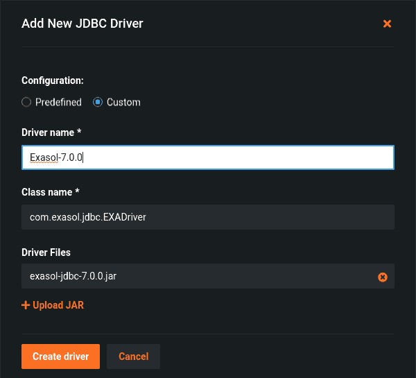
You’ll need to:

• Set the driver name with e.g Exasol-7.0.0
• Add the class name com.exasol.jdbc.EXADriver
• Upload the downloaded Exasol JDBC Driver jar file
• Then finally click to create a driver

Create a DataRobot Exasol Connection

• Open the DataRobot user interface and go to the AI Catalog
• Click the “Add to Catalog” button
• Select “New Data Connection”
• Select “My Drivers”

Define the connection

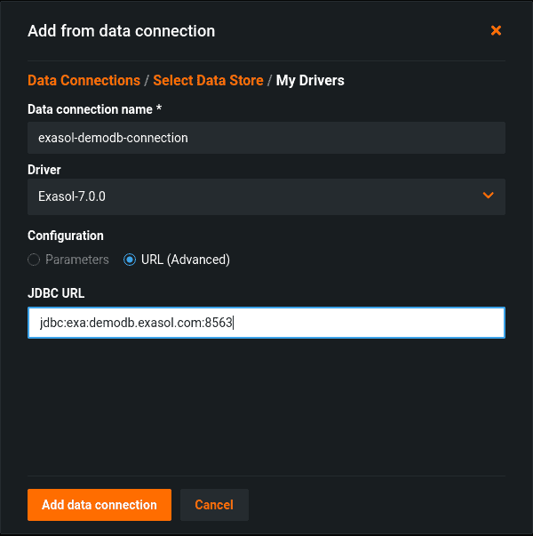
• Give a descriptive name, for example, ExasolConnection
• Choose Exasol JDBC Driver from the Driver section
• Then provide the JDBC connection URL for Exasol database. For this example, we are going to Exasol Demo Database with connection URL as jdbc:exa:demodb.exasol.com:8563. 
• Select “Add Data Connection”

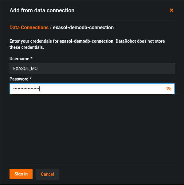
Once you click on the Add Data Connection, DataRobot will ask for your credentials to connect to the database. Please fill in the username and password fields accordingly.

Finally, click on the Sign in button and we can select our dataset and continue to build a DataRobot project with it. 

You can read more about configuration parameters on our Exasol JDBC  documentation.

Import Datasets Into DataRobot

After creating a connection and logging in to the Exasol database, you can choose to import the tables into DataRobot for model building.

To do this:

• Select the Tables tab and search for the datasets you have created earlier.
• Click to proceed with registration.

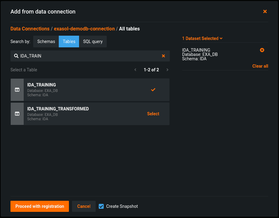
It may take some time to create and register the dataset. Once it’s ready, click on the “Create a project” option to create a new project.

Building your Machine Learning Model Using DataRobot

Now we are at the AutoPilot panel. It can automatically analyze the dataset and discover the informative feature set.

To do this, you’ll need to set a predict target by:

• Selecting the “Class” variable as our target
• And then clicking on the “Start” button to start the AutoPilot.

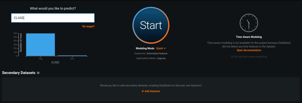
AutoPilot automatically analyzes the dataset and provides detailed information about the feature set. It also automatically starts building several Machine Learning models presenting the best performing models for you.

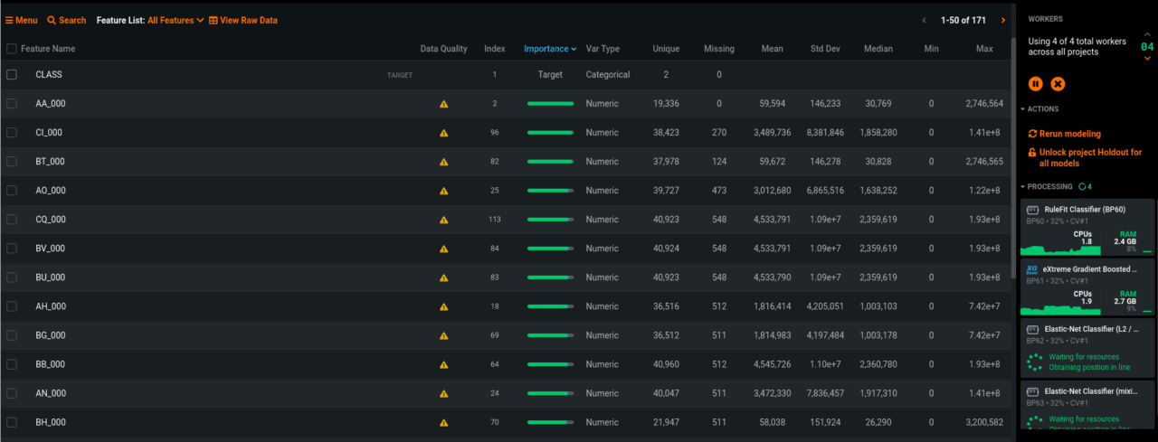
To see the full list of models:

• Select “Models”

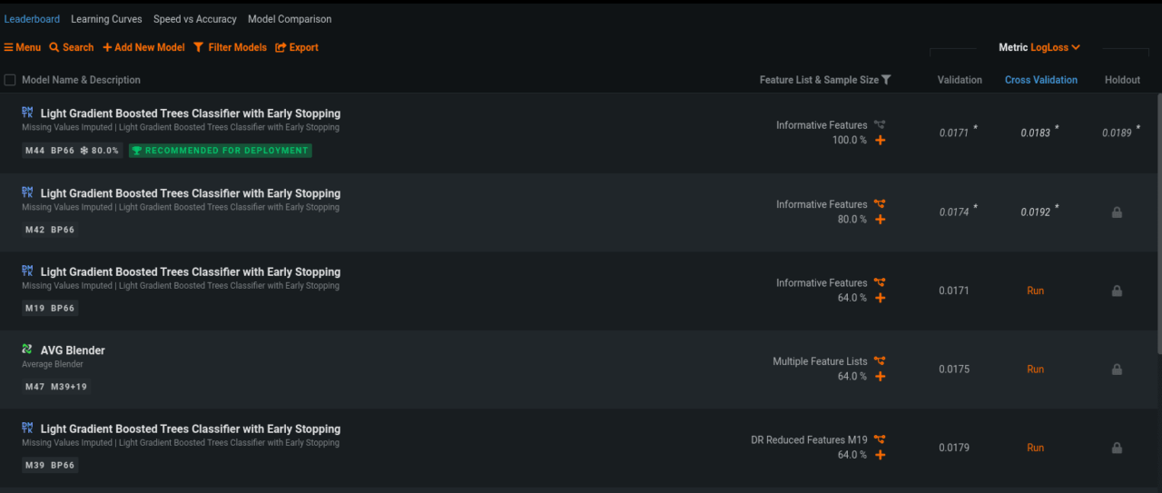
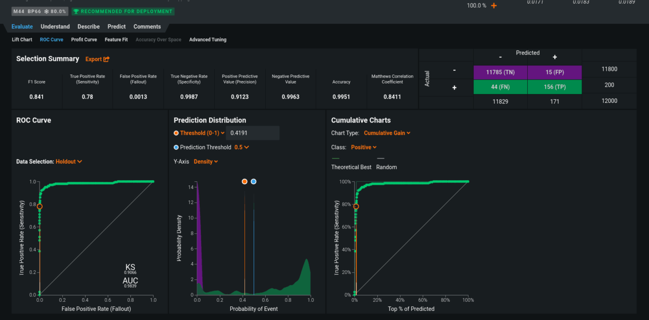
The ranking of these models are based on either accuracy or performance. Each model provides documentation so that you can check out the evaluation or understand which features have the biggest impact on the prediction target.

What next

In this blog post we showed how to use the Exasol database from DataRobot. This allows users to directly access the data from Exasol and transform their data into invaluable machine learning models.

If you want to learn how to call DataRobot prediction calls from Exasol check out the following How-To guide. This approach allows you directly call DataRobot predicitons from your BI frontend. 

For more, check out the DataRobot Platform and Exasol Data Science integration offerings.