Most ML inference architectures have a quiet contradiction at the center. The models live on a GPU somewhere, and the data lives in your warehouse, and the only way they meet is through a pipeline that exports rows, ships them across the network, and waits for predictions to come back. While the mechanism works, it also increases latency, complexity, and governance overhead in a production ML stack.
We wanted to put a number on what happens when you stop moving the data. We scored 15,000 Amazon reviews for sentiment entirely inside Exasol and ran it twice. Once on CPU, once on a GPU-enabled node. The gap between the two runs turned out to be roughly an order of magnitude.

Why exporting data for inference is expensive

The standard pattern is straightforward. Run a query against the warehouse, serialize the result, send it to a model server over the network, get predictions back, and write them somewhere downstream. It works, but it also has costs that don’t show up in any single component.

The first cost is operational. Running inference outside the database means you’re operating two systems that have to stay in sync. The database, where the data lives. The model server, where the model runs. That’s two deployments to maintain, and a contract between them (the export schema and the request format) that breaks whenever one side changes.
The second cost is freshness. When inference runs as a scheduled batch job, the typical setup for warehouse-side ML, predictions are only as current as the last batch finished. That’s fine until a downstream query expects up-to-date scores. The third cost is regulatory. The data leaves the database on every export, which matters whenever the dataset is covered by a compliance regime.

These costs scale with volume. Workloads that run continuously and grow with the business are where the gap between a one-system and two-system architecture shows up first.
In-database inference removes the second system. The model runs on the same node that the SQL query plan invokes, against data that’s already there. No export, no model server, no contract between them.

How Exasol UDFs enable in-database ML

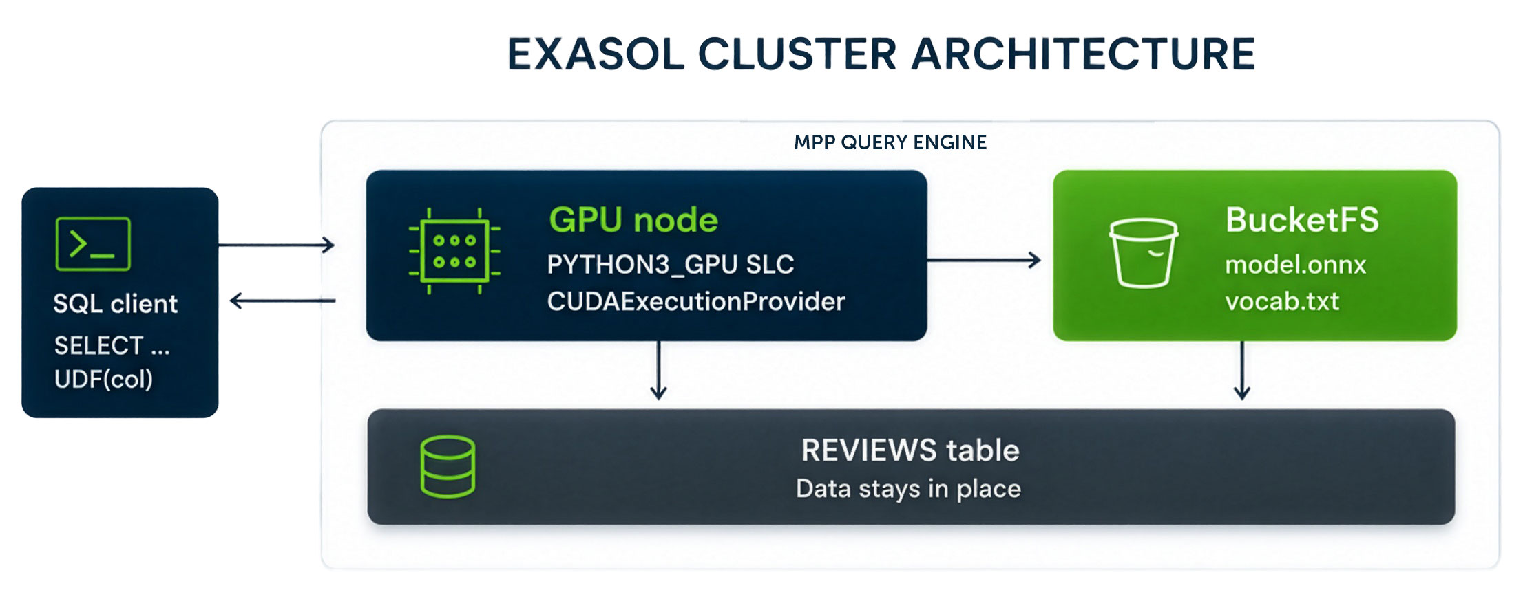
A User-Defined Function (UDF) in Exasol is a script that runs inside the database engine. When you call a UDF in a SQL query, Exasol’s MPP architecture distributes execution across Exasol’s cluster’s compute nodes. Each node processes its partition of the data in parallel, and results flow back into the query plan as just another column.

SELECT
    REVIEW_TEXT,
    ML_SCHEMA.SENTIMENT_GPU(REVIEW_TEXT) AS PREDICTED_LABEL
FROM ML_SCHEMA.REVIEWS;

A Script Language Container (SLC) is the Linux container image that the UDF executes in. It bundles the Python interpreter and its libraries into one image, so every node in the cluster runs the same environment. The default SLC includes the common data science libraries. If you need something extra (ONNX Runtime, transformers, a specific scikit-learn version), you add it to the SLC and rebuild.
For GPU work, Exasol publishes a CUDA-enabled flavor called template-Exasol-8-python-3.10-cuda-conda. The benchmark loads it under the PYTHON3_GPU language alias, which is the name the UDF references in SQL. The UDF code stays the same. Only the container image changes. The architecture keeps the model, the data, and the compute in the same place. No model server or external orchestrator. No serialization tier in between.

Why GPU acceleration changes the performance ceiling

CPUs handle transformer inference, but they do it sequentially. The forward pass through an AI model is a chain of matrix multiplications, and that is exactly what GPUs are built to accelerate. On a single review, the difference is small enough not to matter. Across 15,000 reviews, it compounds into the 10× gap seen in the GPU run.

Two terms matter here, both from ONNX Runtime’s provider system:

• CPUExecutionProvider: The default backend. Each row is tokenized, the model runs its forward pass on the CPU, and the predictions return.
• CUDAExecutionProvider: The same forward pass, dispatched to NVIDIA CUDA kernels. Tokenized inputs are copied to GPU memory, computed, and the result is returned.

Switching between execution providers requires a GPU-enabled node in the cluster. For this benchmark, we used an AWS g4dn.xlarge with an NVIDIA T4. In the UDF’s CREATE SCRIPT statement, the PYTHON3_GPU language alias selects which activated SLC will run the UDF. The %perInstanceRequiredAcceleratorDevices option parameter declares whether the UDF requires or prefers a GPU, and Exasol uses that declaration to schedule the work on a node with the right hardware.

Exasol UDFs are defined by two things: an input type and an output type. The input type, SCALAR or SET, controls how rows are fed to the UDF. The output type, RETURNS or EMITS, controls what comes back. The benchmark uses SCALAR RETURNS for the CPU UDF and SET EMITS for the GPU UDF.

A SCALAR UDF is called once per row by the SQL planner. The function receives that row, runs its logic, and produces an output. With RETURNS, the output is one value per row, which is why a SCALAR RETURNS UDF behaves like a regular SQL function (UPPER(name), LENGTH(text)). The planner streams rows through it. It’s the simplest setup and the right one for most CPU work.

A SET UDF is called once per group of rows. The function receives an iterator and can pull as many rows from it as it wants. With EMITS, it can produce any number of output rows. You’d use this combination when the per-row logic isn’t independent, when the function needs to see multiple rows together to do something useful.

GPUs need batches. A single matrix multiplication on a GPU is barely faster than on a CPU because moving the inputs into GPU memory and launching a CUDA kernel both have fixed costs. You get real gains by running many forward passes at once. For example, 64 tokenized inputs can be sent in one call and processed in parallel by the GPU’s thousands of cores, then returned together. The kernel launch overhead is paid once, the parallelism is fully used, and the per row cost drops by an order of magnitude.

A scalar UDF on the GPU would call the ONNX session.run() once per row, paying the kernel-launch overhead 15,000 times for 15,000 rows. The GPU would sit idle between invocations. The right shape is a SET UDF. It accumulates rows into a buffer of 64, calls session.run() once per buffer, and lets the GPU do all 64 forward passes in parallel. The kernel-launch overhead is paid 235 times instead of 15,000.

One Exasol-specific note. A SET script always needs a GROUP BY clause to tell Exasol how to divide the rows. The benchmark uses GROUP BY IPROC(). 

SELECT ML_SCHEMA.SENTIMENT_GPU_BATCH(REVIEW_TEXT, TRUE_LABEL)
FROM   ML_SCHEMA.REVIEWS
GROUP BY IPROC();

IPROC() is an Exasol built-in that returns the node number for each row, so this clause means “give each node its own group of rows.” In a multi-node cluster, each node would receive its own SET-script invocation, running on its own GPU, using data already stored locally on that node. That’s how the same SQL scales out without rewriting it. 

In our single-node setup, every row reports node 0, so there’s a single group and a single invocation. The 10× speedup we measured comes entirely from GPU batching inside that one invocation. Adding more nodes is the next step up. 

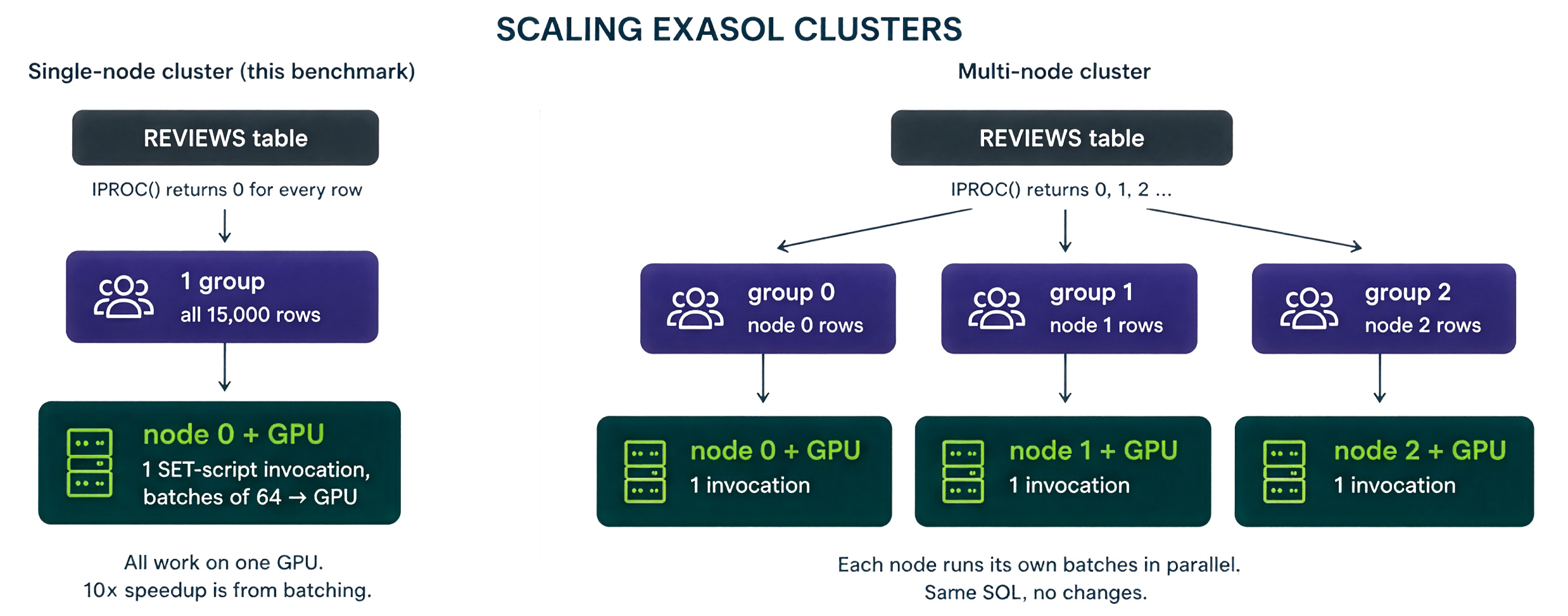
That is the architecture. Same model file, same tokenizer, same SQL surface. A different UDF shape and a different execution provider, with two layers of parallelism stacked on top of each other.

Benchmark methodology

The benchmark compared two UDFs running the same model on the same data, varying only the execution provider. A retailer wants sentiment scores like positive, neutral, or negative on its product reviews so downstream queries can filter, aggregate, and chart by sentiment alongside the rest of the review data. The setup is documented below.

Workload

The benchmark uses 15,000 Amazon product reviews as the test set. DistilBERT (distilbert-base-uncased) was fine-tuned for three-class sentiment classification on the dataset and exported to ONNX. Both UDFs load the same model. Tokenization, preprocessing, and max_length=128 are identical across runs. The only variable is the execution provider.

Hardware

• AWS g4dn.xlarge: 4 vCPUs, 16 GB RAM
• NVIDIA T4 GPU, 16 GB memory

Software

• Exasol 2025.2.1
• ONNX Runtime 1.23.2 (GPU build, nvidia-cudnn-cu12)
• Ubuntu 22.04, NVIDIA driver 535+
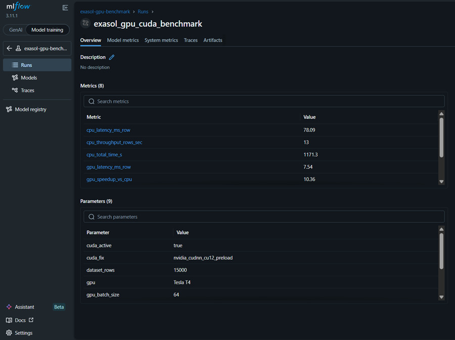
• MLflow for run tracking under the exasol-gpu-benchmark experiment

Scalar on CPU, batched on GPU

Scalar UDFs process one row at a time, which is how they’re called from SQL. The GPU UDF batches at batch_size=64. Each GPU call has a fixed setup cost, so processing one row per call leaves the GPU idle most of the time.[2

Scope

Single node with one T4 GPU. DistilBERT with 67 million parameters. 15,000 rows. Single run. Results will vary with different hardware, sequence lengths, or concurrent workloads.

What the results actually mean

The result is a 10.36× speedup. The CPU run takes over 19 minutes, while the GPU run finishes in under two. The model weights and predictions are the same in both cases. The GPU does not change what the model computes; it only changes how quickly the computation runs.

Metric	CPU UDF	GPU UDF
Total time (15,000 rows)	1,171.3s	113.1s
Throughput	13 rows/sec	133 rows/sec
Per-row latency	78.09 ms	7.54 ms
Predictions match	—	Identical to CPU

Here’s how it shows up in the MLflow dashboard:

Three concrete scenarios where this changes what’s feasible:

• Large-scale review or feedback scoring: An e-commerce platform scoring 200,000 new reviews per day, about 8,300 per hour at peak. At 133 rows/sec, that’s roughly a one-minute SQL job. At 13 rows/sec, it’s over ten. Move the volume up to a million reviews, and the gap goes from “noticeable” to “the difference between a batch job and a multi-day job.”
• Fraud or anomaly checks on transactions: Score transaction text or metadata in the same SQL that the downstream system already runs. The UDF shape and provider switch are the same as the sentiment example. Only the model changes.
• Interactive analytics with embedded scoring: When ML scoring is just a column in a SELECT, you can filter on it directly (WHERE sentiment = ‘negative’). This means, no need to export the data, score it elsewhere, and load it back in.

The infrastructure consequence is what makes this durable. No separate model-serving tier to size, no export pipeline to maintain, no inference-side data egress to monitor. One less moving part in the system, and the part you removed is usually the most failure-prone one.

What can developers do right now?

The reference implementation covers the full stack. Notebooks run in order:

1. dataset_creation.ipynb: pull and prepare the Amazon Reviews data
2. model_finetuning.ipynb: fine-tune DistilBERT, log to MLflow
3. model_export_onnx.ipynb: export to ONNX, generate UDF SQL
4. gpu_benchmark.ipynb: run both UDFs, log results

The implementation includes SLC build tooling, UDF definitions, MLflow tracking config, and SQL scripts for diagnosing CUDA initialization issues. To swap models, export your own to ONNX with optimum[onnxruntime], drop it in BucketFS, and point the UDF at the new path.

Batch size is the main knob worth tuning. The batch size of 64 worked well on the T4. Longer sequences or larger models may need to come down.

We introduced BucketFS above, which is Exasol’s distributed file store, a replicated filesystem inside the cluster that every UDF process can read from without a network hop. The model, tokenizer, and preprocessing are identical across runs.

Conclusion

The benchmark runs DistilBERT inference on 15,000 reviews inside Exasol in two modes. The first uses a CPU UDF. The second uses a GPU UDF with batching at 64 rows. Both runs use the same model and the same input data.

The GPU run finishes in 113 seconds, compared to 1,171 seconds on the CPU, with identical predictions. The 10× improvement is the visible result. The more important outcome is architectural.

The data never leaves the database. For datasets governed by GDPR, HIPAA, or internal data classification policies, this removes an entire class of security concerns. There was no network round-trip per row. The model file loads once into the UDF process. Every forward pass runs in the same memory space as the SQL planner that called it. The latency budget is the forward pass itself.

You can apply the same pattern to your own workloads: prepare your dataset, fine-tune or select a model, export it to ONNX, and run the GPU-accelerated UDFs directly inside Exasol. The SQL doesn’t change. If you are new to Exasol, the product overview is the right place to start.