SQL Data Warehouse in SQL Server: Design, Build & Optimize

A SQL data warehouse is a database designed for analytical queries, typically using a star schema with fact and dimension tables. In SQL Server, a DWH combines staging, ETL, and optimized storage (partitioning, columnstore) to support reporting and analytics at scale.

The term SQL Data Warehouse is used in different ways, which often creates confusion. In Microsoft documentation, it can refer to the Management Data Warehouse (MDW) — a repository that stores performance data for monitoring SQL Server instances. In Azure, it was the original name of the Dedicated SQL Pool in Synapse Analytics, a massively parallel processing (MPP) service for large-scale analytical workloads. In practice, many professionals also use the term when they build a star-schema analytical data warehouse on SQL Server itself, using features such as columnstore indexes and partitioned tables.

Each of these approaches builds on general principles of data warehouse architecture, but the technologies, use cases, and costs differ. This page explains all three meanings, shows how SQL Server can serve as a data warehouse platform, and compares it with Azure Synapse and Exasol. It includes a practical walkthrough, dimensional modeling patterns, performance guidance, and a comparison matrix to help you select the right technology for your environment.

What Does “SQL Data Warehouse” Mean?

The phrase SQL Data Warehouse appears in three distinct contexts. Understanding the differences is critical because they involve separate technologies and use cases.

SQL Server Management Data Warehouse (MDW)

The Management Data Warehouse is a SQL Server feature for collecting and storing performance metrics. It captures data from the Data Collector and writes it into a repository database. Administrators use it to monitor resource usage, query statistics, and server health. It is not designed for analytics or reporting across business domains.

Azure Synapse Dedicated SQL Pool

The service once branded as Azure SQL Data Warehouse is now called the Dedicated SQL Pool in Azure Synapse Analytics. It uses a massively parallel processing (MPP) architecture where compute and storage scale independently. This model supports analytical workloads on terabytes or petabytes of data. Users can pause or resume compute resources and integrate directly with other Azure services such as Power BI or Azure Machine Learning.

SQL Server as an Analytical Data Warehouse

SQL Server itself can be configured as a data warehouse platform. Typical implementations follow a star schema with fact and dimension tables. Features such as clustered columnstore indexes, table partitioning, and integration with SQL Server Integration Services (SSIS) allow it to handle analytical queries at moderate scale. Many organizations start with SQL Server because it leverages existing licensing, skills, and infrastructure.

These implementations share many of the same design principles described in our overview of data warehouse concepts.

SQL Server vs Azure Synapse vs Exasol

The three technologies differ in architecture, performance model, and cost. The table below summarizes the core distinctions.

Technology	Architecture	Strenghts	Best For	Cost Model
SQL Server (on-prem)	Single-node RDBMS with parallel query support	Familiar toolchain, wide ecosystem, strong OLTP/OLAP integration	Organizations with existing SQL Server licenses, moderate-scale analytics	Per-core or server license + on-prem infrastructure
Azure Synapse Dedicated SQL Pool	Cloud-native MPP (compute nodes + control node) with separated storage	Elastic scaling, direct Azure ecosystem integration (Power BI, ML, Data Factory)	Enterprises running large-scale cloud analytics, variable workloads	Consumption-based pricing per DWU (data warehouse unit)
Exasol	In-memory, massively parallel processing (MPP), vectorized execution	Very high query performance, advanced compression, sovereignty-friendly deployment	Analytics-driven businesses needing fast reporting and hybrid or regulated environments	Subscription, flexible deployment (on-prem, cloud, hybrid)

When to Choose Each

SQL Server (on-prem)

Choose SQL Server when you already run Microsoft workloads on-premises and need to extend them into analytics without adding new platforms. It is practical for mid-sized data warehouses where fact tables remain in the hundreds of millions of rows rather than tens of billions. Existing licenses, skills, and infrastructure lower adoption cost.

Azure Synapse Dedicated SQL Pool

Select Synapse when your data strategy is cloud-first and tightly integrated with Azure services. It suits workloads that require elastic compute — for example, variable reporting peaks, proof-of-concept projects, or analytics where storage grows faster than compute demand. Dedicated SQL Pool supports petabyte-scale data, but carries the overhead of Azure lock-in and consumption billing.

Exasol

Use Exasol Analytics Engine when query speed and analytical concurrency are critical. Its in-memory MPP design makes it well suited for organizations with hundreds of BI users or real-time analytical dashboards. It also fits regulated industries that need sovereignty options, as it runs on-prem, in private cloud, or in hybrid deployments.

Building a SQL Server Data Warehouse (Practical Walkthrough)

Goal: Stand up a small, star-schema warehouse on SQL Server (Express or Developer for non-production) using sample data (e.g., AdventureWorks). Steps: model → create DB/schemas → stage/load → transform to facts/dimensions → optimize → validate → operate.

Quick prerequisites (so the scripts run)

• Edition/Version:
  • SQL Server 2016 SP1+: Columnstore and table partitioning are available in all editions (incl. Express/Developer).
  • Earlier than 2016 SP1: Partitioning and columnstore may require Enterprise. If unavailable, skip the partitioning section and keep a rowstore table.
• Sample data: If you have AdventureWorks OLTP on the same instance, use Option A loads. If you only have CSVs, use Option B BULK INSERT (choose ROWTERMINATOR that matches your files: ‘\r\n’ for Windows CSVs, ‘\n’ for Unix).

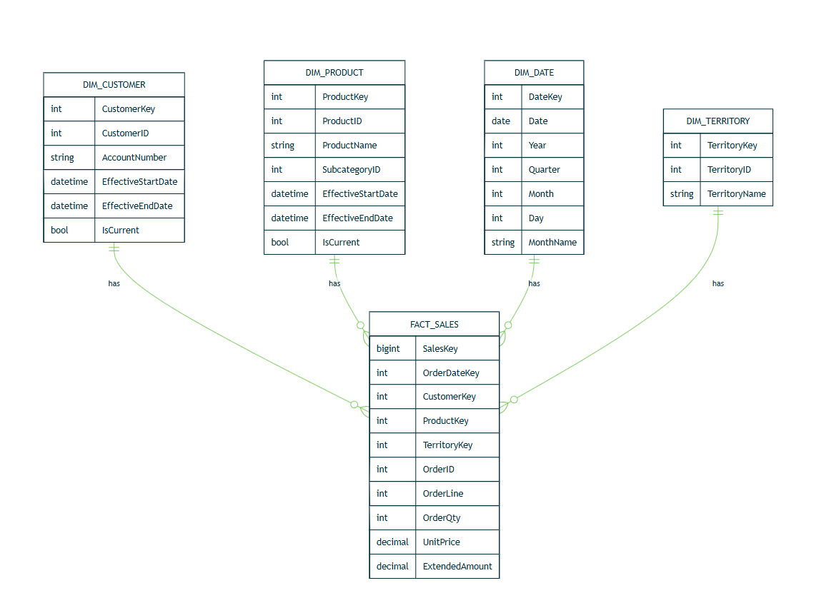
Schema Design with AdventureWorks

Before creating objects, define the data warehouse grain and identify fact and dimension tables. In this walkthrough, we use AdventureWorks as the source model.

Star schema

• Dimensions (examples): dimDate, dimCustomer, dimProduct, dimTerritory.
• Facts (examples): factSales (grain: one line per sales order detail).
• Keys: Integer surrogate keys on dimensions; foreign keys in facts.
• Auditing columns: CreatedAt, UpdatedAt, SourceSystem.

Source → Target mapping (sample)

• Sales.SalesOrderHeader + Sales.SalesOrderDetail → factSales
• Sales.Customer (+ person/account tables as needed) → dimCustomer
• Production.Product (+ subcategory/category) → dimProduct
• Calendar table generated → dimDate

Database Setup and Schemas

The data warehouse is created in its own database with separate schemas (stage, dim, fact) and security roles for ETL and BI access.

IF DB_ID('DW_SQLServer') IS NULL
    CREATE DATABASE DW_SQLServer;
GO
USE DW_SQLServer;
GO

IF NOT EXISTS (SELECT 1 FROM sys.schemas WHERE name = 'stage') EXEC('CREATE SCHEMA stage');
IF NOT EXISTS (SELECT 1 FROM sys.schemas WHERE name = 'dim')   EXEC('CREATE SCHEMA dim');
IF NOT EXISTS (SELECT 1 FROM sys.schemas WHERE name = 'fact')  EXEC('CREATE SCHEMA fact');
GO

IF NOT EXISTS (SELECT 1 FROM sys.database_principals WHERE name = 'etl_role') CREATE ROLE etl_role;
IF NOT EXISTS (SELECT 1 FROM sys.database_principals WHERE name = 'bi_role')  CREATE ROLE bi_role;

GRANT SELECT, INSERT, UPDATE, DELETE ON SCHEMA::stage TO etl_role;
GRANT SELECT ON SCHEMA::dim  TO bi_role;
GRANT SELECT ON SCHEMA::fact TO bi_role;
GO

Staging and Loading

Raw data is first copied into staging tables, either by INSERT … SELECT from AdventureWorks or by BULK INSERT from CSV files.

Staging tables

IF OBJECT_ID('stage.SalesOrderHeader','U') IS NOT NULL DROP TABLE stage.SalesOrderHeader;
IF OBJECT_ID('stage.SalesOrderDetail','U') IS NOT NULL DROP TABLE stage.SalesOrderDetail;
IF OBJECT_ID('stage.Customer','U')        IS NOT NULL DROP TABLE stage.Customer;
IF OBJECT_ID('stage.Product','U')         IS NOT NULL DROP TABLE stage.Product;
IF OBJECT_ID('stage.Territory','U')       IS NOT NULL DROP TABLE stage.Territory;

CREATE TABLE stage.SalesOrderHeader (
  SalesOrderID INT,
  OrderDate    DATE,
  CustomerID   INT,
  TerritoryID  INT
);
CREATE TABLE stage.SalesOrderDetail (
  SalesOrderID        INT,
  SalesOrderDetailID  INT,
  ProductID           INT,
  OrderQty            INT,
  UnitPrice           DECIMAL(19,4)
);
CREATE TABLE stage.Customer (
  CustomerID    INT,
  AccountNumber NVARCHAR(25)
);
CREATE TABLE stage.Product (
  ProductID            INT,
  Name                 NVARCHAR(200),
  ProductSubcategoryID INT NULL
);
CREATE TABLE stage.Territory (
  TerritoryID INT,
  Name        NVARCHAR(100)
);

Bulk load (if your CSVs are standard Windows files → use ‘\r\n’)

BULK INSERT stage.SalesHeader
FROM 'C:\data\SalesOrderHeader.csv'
WITH (FIRSTROW=2, FIELDTERMINATOR=',', ROWTERMINATOR = '\r\n', TABLOCK);

BULK INSERT stage.SalesDetail
FROM 'C:\data\SalesOrderDetail.csv'
WITH (FIRSTROW=2, FIELDTERMINATOR=',', ROWTERMINATOR = '\r\n', TABLOCK);

BULK INSERT stage.Customer
FROM 'C:\data\Customer.csv'
WITH (FIRSTROW=2, FIELDTERMINATOR=',', ROWTERMINATOR = '\r\n', TABLOCK);

BULK INSERT stage.Product
FROM 'C:\data\Product.csv'
WITH (FIRSTROW=2, FIELDTERMINATOR=',', ROWTERMINATOR = '\r\n', TABLOCK);

BULK INSERT stage.Territory
FROM 'C:\data\Territory.csv'
WITH (FIRSTROW=2, FIELDTERMINATOR=',', ROWTERMINATOR = '\r\n', TABLOCK);

(If pulling directly from AdventureWorks within the same instance, replace BULK INSERT with INSERT … SELECT from source tables.)

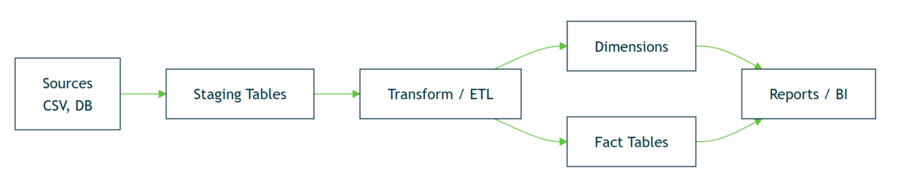
The high-level ETL flow looks like this before we dive into SQL examples:

Dimension Tables

Dimension tables store descriptive attributes and are loaded from staging with surrogate keys and optional Slowly Changing Dimension (SCD) handling.

Date dimension (generated)

IF OBJECT_ID('dim.[Date]','U')    IS NOT NULL DROP TABLE dim.[Date];
IF OBJECT_ID('dim.Customer','U')  IS NOT NULL DROP TABLE dim.Customer;
IF OBJECT_ID('dim.Product','U')   IS NOT NULL DROP TABLE dim.Product;
IF OBJECT_ID('dim.Territory','U') IS NOT NULL DROP TABLE dim.Territory;
GO

CREATE TABLE dim.[Date] (
  DateKey      INT          NOT NULL PRIMARY KEY,  -- YYYYMMDD
  [Date]       DATE         NOT NULL UNIQUE,
  [Year]       SMALLINT     NOT NULL,
  [Quarter]    TINYINT      NOT NULL,
  [Month]      TINYINT      NOT NULL,
  [Day]        TINYINT      NOT NULL,
  MonthName    NVARCHAR(15) NOT NULL,
  QuarterName  AS (CONCAT('Q', [Quarter]))
);
GO
DECLARE @d0 DATE='2022-01-01', @d1 DATE='2026-12-31';
;WITH n AS (
  SELECT TOP (DATEDIFF(DAY,@d0,@d1)+1)
         ROW_NUMBER() OVER (ORDER BY (SELECT 1)) - 1 AS i
  FROM sys.all_objects
)
INSERT INTO dim.[Date] (DateKey,[Date],[Year],[Quarter],[Month],[Day],MonthName)
SELECT CONVERT(INT, CONVERT(CHAR(8), DATEADD(DAY,i,@d0), 112)),
       DATEADD(DAY,i,@d0),
       DATEPART(YEAR,  DATEADD(DAY,i,@d0)),
       DATEPART(QUARTER,DATEADD(DAY,i,@d0)),
       DATEPART(MONTH, DATEADD(DAY,i,@d0)),
       DATEPART(DAY,   DATEADD(DAY,i,@d0)),
       DATENAME(MONTH, DATEADD(DAY,i,@d0));
GO

CREATE TABLE dim.Customer (
  CustomerKey         INT IDENTITY(1,1) PRIMARY KEY,
  CustomerID          INT           NOT NULL UNIQUE,
  AccountNumber       NVARCHAR(25)  NULL,
  EffectiveStartDate  DATETIME2     NOT NULL DEFAULT SYSUTCDATETIME(),
  EffectiveEndDate    DATETIME2     NULL,
  IsCurrent           BIT           NOT NULL DEFAULT 1
);
CREATE TABLE dim.Product (
  ProductKey          INT IDENTITY(1,1) PRIMARY KEY,
  ProductID           INT           NOT NULL UNIQUE,
  ProductName         NVARCHAR(200) NOT NULL,
  SubcategoryID       INT           NULL,
  EffectiveStartDate  DATETIME2     NOT NULL DEFAULT SYSUTCDATETIME(),
  EffectiveEndDate    DATETIME2     NULL,
  IsCurrent           BIT           NOT NULL DEFAULT 1
);
CREATE TABLE dim.Territory (
  TerritoryKey  INT IDENTITY(1,1) PRIMARY KEY,
  TerritoryID   INT           NOT NULL UNIQUE,
  TerritoryName NVARCHAR(100) NOT NULL
);
GO

-- Initial loads
INSERT INTO dim.Customer (CustomerID, AccountNumber)
SELECT DISTINCT CustomerID, AccountNumber FROM stage.Customer;

INSERT INTO dim.Product (ProductID, ProductName, SubcategoryID)
SELECT DISTINCT ProductID, Name, ProductSubcategoryID FROM stage.Product;

INSERT INTO dim.Territory (TerritoryID, TerritoryName)
SELECT DISTINCT TerritoryID, Name FROM stage.Territory;
GO

Customer, Product, Territory (surrogate keys)

CREATE TABLE dim.Customer (
  CustomerKey INT IDENTITY(1,1) PRIMARY KEY,
  CustomerID INT UNIQUE,        -- business/natural key
  AccountNumber NVARCHAR(20),
  EffectiveStartDate DATETIME2 NOT NULL DEFAULT SYSUTCDATETIME(),
  EffectiveEndDate DATETIME2 NULL,
  IsCurrent BIT NOT NULL DEFAULT 1
);

CREATE TABLE dim.Product (
  ProductKey INT IDENTITY(1,1) PRIMARY KEY,
  ProductID INT UNIQUE,
  ProductName NVARCHAR(200),
  SubcategoryID INT,
  EffectiveStartDate DATETIME2 NOT NULL DEFAULT SYSUTCDATETIME(),
  EffectiveEndDate DATETIME2 NULL,
  IsCurrent BIT NOT NULL DEFAULT 1
);

CREATE TABLE dim.Territory (
  TerritoryKey INT IDENTITY(1,1) PRIMARY KEY,
  TerritoryID INT UNIQUE,
  TerritoryName NVARCHAR(100)
);

Initial dimension load (simplified, no SCD yet)

INSERT INTO dim.Customer (CustomerID, AccountNumber)
SELECT DISTINCT CustomerID, AccountNumber
FROM stage.Customer;

INSERT INTO dim.Product (ProductID, ProductName, SubcategoryID)
SELECT DISTINCT ProductID, Name, ProductSubcategoryID
FROM stage.Product;

INSERT INTO dim.Territory (TerritoryID, TerritoryName)
SELECT DISTINCT TerritoryID, Name
FROM stage.Territory;

Fact Table

The fact table captures sales events, with foreign keys to each dimension and measures such as OrderQty, UnitPrice, and ExtendedAmount.

IF OBJECT_ID('fact.Sales','U') IS NOT NULL DROP TABLE fact.Sales;
GO

-- Partitioning (optional; remove ON clause below if not supported)
IF NOT EXISTS (SELECT 1 FROM sys.partition_functions WHERE name='pf_SalesDate')
BEGIN
  CREATE PARTITION FUNCTION pf_SalesDate (INT)
  AS RANGE RIGHT FOR VALUES (20220101, 20220201, 20220301, 20220401, 20220501, 20220601);
END
IF NOT EXISTS (SELECT 1 FROM sys.partition_schemes WHERE name='ps_SalesDate')
BEGIN
  CREATE PARTITION SCHEME ps_SalesDate
  AS PARTITION pf_SalesDate ALL TO ([PRIMARY]);
END
GO

CREATE TABLE fact.Sales (
  SalesKey      BIGINT IDENTITY(1,1) NOT NULL,
  OrderDateKey  INT    NOT NULL,
  CustomerKey   INT    NOT NULL,
  ProductKey    INT    NOT NULL,
  TerritoryKey  INT    NOT NULL,
  OrderID       INT    NOT NULL,
  OrderLine     INT    NOT NULL,
  OrderQty      INT    NOT NULL,
  UnitPrice     DECIMAL(19,4) NOT NULL,
  ExtendedAmount AS (OrderQty * UnitPrice) PERSISTED,
  CONSTRAINT PK_Sales PRIMARY KEY NONCLUSTERED (SalesKey),
  CONSTRAINT FK_Sales_Date      FOREIGN KEY (OrderDateKey)  REFERENCES dim.[Date](DateKey),
  CONSTRAINT FK_Sales_Customer  FOREIGN KEY (CustomerKey)   REFERENCES dim.Customer(CustomerKey),
  CONSTRAINT FK_Sales_Product   FOREIGN KEY (ProductKey)    REFERENCES dim.Product(ProductKey),
  CONSTRAINT FK_Sales_Territory FOREIGN KEY (TerritoryKey)  REFERENCES dim.Territory(TerritoryKey)
) ON ps_SalesDate (OrderDateKey);  -- delete this clause if not partitioning
GO

Key lookups and load

The fact table is populated by joining staged headers and details to dimension keys, with dates converted to integer DateKey values.

;WITH hdr AS (
  SELECT SalesOrderID, OrderDate, CustomerID, TerritoryID
  FROM stage.SalesOrderHeader
),
det AS (
  SELECT SalesOrderID, SalesOrderDetailID, ProductID, OrderQty, UnitPrice
  FROM stage.SalesOrderDetail
)
INSERT INTO fact.Sales (
  OrderDateKey, CustomerKey, ProductKey, TerritoryKey,
  OrderID, OrderLine, OrderQty, UnitPrice
)
SELECT
  CONVERT(INT, CONVERT(CHAR(8), h.OrderDate, 112)) AS OrderDateKey,
  dc.CustomerKey,
  dp.ProductKey,
  dt.TerritoryKey,
  d.SalesOrderID,
  d.SalesOrderDetailID,
  d.OrderQty,
  d.UnitPrice
FROM det d
JOIN hdr h ON h.SalesOrderID = d.SalesOrderID
JOIN dim.Customer  dc ON dc.CustomerID  = h.CustomerID AND dc.IsCurrent = 1
JOIN dim.Product   dp ON dp.ProductID   = d.ProductID  AND dp.IsCurrent = 1
JOIN dim.Territory dt ON dt.TerritoryID = h.TerritoryID;
GO

Performance Enhancements

Large analytical queries in SQL Server benefit from dedicated features that optimize storage and execution. Independent research, such as the Star Schema Benchmark, has shown how schema design and indexing choices can directly influence analytical query performance.

In contrast, organizations like Piedmont Healthcare have migrated off SQL Server and onto Exasol, with a remarkable up to 1,000× performance improvement, entire data mart refreshes cut from hours to minutes, and query response times reduced from 10 minutes to seconds. This real-world example underscores the upper ceiling of performance that modern analytical engines like Exasol enable.

Clustered columnstore index on fact

Columnstore indexing stores data in compressed column segments, improving scan and aggregation performance.

-- Create clustered columnstore AFTER initial load
IF NOT EXISTS (
  SELECT 1 FROM sys.indexes WHERE name='CCI_FactSales' AND object_id=OBJECT_ID('fact.Sales')
)
  CREATE CLUSTERED COLUMNSTORE INDEX CCI_FactSales ON fact.Sales;

Building CCI after the load produces optimal compressed rowgroups and avoids fragmentation.

Partitioning (by OrderDateKey, monthly example)

Partitioning spreads data across multiple slices. Queries can eliminate partitions based on filters, improving performance.

CREATE PARTITION FUNCTION pf_SalesDate (INT)
AS RANGE RIGHT FOR VALUES (20220101, 20220201, 20220301, 20220401, 20220501, 20220601);

CREATE PARTITION SCHEME ps_SalesDate
AS PARTITION pf_SalesDate ALL TO ([PRIMARY]);

CREATE TABLE fact.Sales (
  -- columns...
) ON ps_SalesDate (OrderDateKey);   -- <— required

(If you’re early in the build, define partitioning before loading. For existing data, use SWITCH PARTITION to migrate with minimal downtime.)

Validation Queries

-- Rows by month (fast INT math)
SELECT (OrderDateKey / 100) AS YYYYMM, COUNT(*) AS RowCount
FROM fact.Sales
GROUP BY (OrderDateKey / 100)
ORDER BY YYYYMM;

-- Top customers by revenue
SELECT TOP (10) c.AccountNumber, SUM(s.ExtendedAmount) AS Revenue
FROM fact.Sales s
JOIN dim.Customer c ON s.CustomerKey = c.CustomerKey
GROUP BY c.AccountNumber
ORDER BY Revenue DESC;

-- Product by territory
SELECT t.TerritoryName, p.ProductName, SUM(s.ExtendedAmount) AS Revenue
FROM fact.Sales s
JOIN dim.Territory t ON s.TerritoryKey = t.TerritoryKey
JOIN dim.Product  p ON s.ProductKey = p.ProductKey
GROUP BY t.TerritoryName, p.ProductName
ORDER BY t.TerritoryName, Revenue DESC;

Batch Mode Execution

Columnstore indexes enable batch mode execution, which processes rows in vectors rather than one by one. No code required; this happens automatically when queries touch columnstore segments.

Parallelism

SQL Server’s cost-based optimizer uses multiple CPU cores for fact-table queries. To maximize throughput:

• Ensure MAXDOP is not forced to 1 unless necessary.
• Keep statistics updated (sp_updatestats) so the optimizer makes accurate decisions.

Operations and Maintenance

After loading, columnstore indexes require periodic maintenance, statistics should be refreshed, and query performance monitored through DMVs or Query Store.

After loading, columnstore indexes require periodic maintenance, statistics should be refreshed, and query performance monitored through DMVs or Query Store.

Index and columnstore maintenance (sample cadence)

-- Columnstore upkeep
ALTER INDEX CCI_FactSales ON fact.Sales REORGANIZE WITH (COMPRESS_ALL_ROW_GROUPS = ON);

-- Occasional rebuild (e.g., after large deletes)
-- ALTER INDEX CCI_FactSales ON fact.Sales REBUILD;

-- Update stats after big loads
EXEC sp_updatestats;

Statistics

-- Update statistics after large loads
EXEC sp_updatestats;

Read-only filegroups (historical partitions)

• Place closed, historical partitions into a filegroup set to READ_ONLY.
• Benefits: faster backups of current data, reduced maintenance overhead.

Monitoring (DMVs)

Dynamic Management Views (DMVs) expose query and storage behavior.

-- Rowgroup health
SELECT * FROM sys.dm_db_column_store_row_group_physical_stats;

-- Waits snapshot
SELECT * FROM sys.dm_os_wait_stats ORDER BY wait_time_ms DESC;

-- Query store (if enabled) for regressed plans
-- Configure Query Store in DW_SQLServer and track top queries by duration/CPU.

Dimensional Modeling in SQL Server

Analytical data warehouses often use a star schema, where fact tables record business events and dimension tables provide descriptive context. SQL Server supports this model with native features such as surrogate keys, temporal tables, and columnstore indexing.

These techniques align with general data warehouse models and approaches, but are implemented in SQL Server with specific features such as MERGE and system-versioned temporal tables. For broader methodology, see the Kimball techniques for dimensional modeling, which remain widely referenced in enterprise data warehousing.

While these modeling best practices help optimize SQL Server, Exasol’s architecture allows for simplified SCD handling and fast computation of derived metrics at scale, as seen in the Piedmont Healthcare deployment, which powers intensive dashboards across 1.8 trillion data points while supporting 20 new metrics per month.

Slowly Changing Dimensions (Type 2 with MERGE)

For dimensions that track historical changes (e.g., a customer changing territories), a Type-2 Slowly Changing Dimension (SCD-2) pattern is common. In SQL Server, MERGE can manage current vs historical rows.

MERGE dim.Customer AS tgt
USING (
  SELECT CustomerID, AccountNumber
  FROM stage.Customer
) AS src
ON (tgt.CustomerID = src.CustomerID AND tgt.IsCurrent = 1)

WHEN MATCHED AND tgt.AccountNumber <> src.AccountNumber
THEN
  -- expire old version
  UPDATE SET tgt.IsCurrent = 0,
             tgt.EffectiveEndDate = SYSUTCDATETIME()

WHEN NOT MATCHED BY TARGET
THEN
  -- insert new customer
  INSERT (CustomerID, AccountNumber, EffectiveStartDate, IsCurrent)
  VALUES (src.CustomerID, src.AccountNumber, SYSUTCDATETIME(), 1)

WHEN NOT MATCHED BY SOURCE
THEN
  -- optional: handle deletes
  UPDATE SET tgt.IsCurrent = 0,
             tgt.EffectiveEndDate = SYSUTCDATETIME();

Notes:

• EffectiveStartDate and EffectiveEndDate track validity windows.
• IsCurrent simplifies joins from the fact table.
• Deletes are optional, depending on retention rules.

Temporal Tables for History Tracking

SQL Server also supports system-versioned temporal tables. These automatically record row changes without manual MERGE logic.

CREATE TABLE dim.Product (
  ProductKey       INT IDENTITY(1,1) PRIMARY KEY,
  ProductID        INT NOT NULL UNIQUE,
  ProductName      NVARCHAR(200) NOT NULL,
  SubcategoryID    INT NULL,
  ValidFrom        DATETIME2 GENERATED ALWAYS AS ROW START NOT NULL,
  ValidTo          DATETIME2 GENERATED ALWAYS AS ROW END   NOT NULL,
  PERIOD FOR SYSTEM_TIME (ValidFrom, ValidTo)
) WITH (SYSTEM_VERSIONING = ON (HISTORY_TABLE = dim.ProductHistory));

Notes:

• Use temporal tables when you want automatic change history.
• They increase storage usage; MERGE offers more control.

Surrogate Keys and Degenerate Dimensions

Surrogate keys (integers) simplify joins and provide stability when natural keys change. In our model, CustomerKey, ProductKey, and TerritoryKey are surrogates.

Degenerate dimensions store identifiers that have no additional attributes (e.g., OrderID in the fact table). These are kept in the fact table rather than creating a separate dimension.

ETL Orchestration Options

• SQL Server Integration Services (SSIS): on-prem ETL tool, suitable for batch pipelines.
• Azure Data Factory (ADF): cloud-native orchestration for hybrid environments.
• dbt: modern ELT framework that executes SQL transformations directly in the data warehouse, often used for analytics-focused teams.

Wrapping Up

Building a SQL data warehouse in SQL Server is a valuable exercise in mastering schemas, staging, transformations, and performance tricks. But as data volumes and user demands grow, tuning alone often hits a ceiling. That’s why companies like Piedmont Healthcare moved from SQL Server to Exasol, unlocking 1,000× faster analytics and the ability to deliver new insights at scale.

⚠️ Note on the code: The SQL shown here is for educational purposes, with a few intentional “Easter eggs” left in. They’re designed to make you pause, think, and validate before running anything in production.

In short: learn the mechanics in SQL Server, but keep an eye on where you’ll need to go next. The real win isn’t just building a data warehouse; it’s choosing a platform that keeps up with your ambitions.

FAQs