How 5 Databases Actually Scale across Concurrency, Data, and Nodes

1. The Question Nobody Tests Publicly

Your data doubled last quarter. Your team grew. Do you buy a bigger machine, or do you add more machines? Every vendor slide deck shows the same chart: a perfectly straight diagonal line labeled “linear scalability.” I have never seen a vendor slide that shows what happens when things go wrong.

I wanted actual numbers. Not theoretical throughput on a workload designed for that engine, but the same 22 TPC-H queries running on the same hardware across five analytical database systems, scaling three dimensions independently: concurrent users, data volume, and cluster size. Twelve configurations total. Within each configuration, every system runs on the same instance type and the same data. Across configurations, hardware scales proportionally with the workload—so ideal behavior is a flat line.

The five systems: Exasol 2025.2.0, ClickHouse 26.1.3.52, StarRocks 4.0.6, Trino 479, and DuckDB 1.4.4. Each is the latest stable release as of February 2026. DuckDB is single-node only, so it participates in concurrency and data scaling but not node scaling.

Disclosure: I work at Exasol as a Principal Architect. Every configuration file, every CSV of raw results, and the complete benchmark framework are published alongside this post. If you think the methodology is flawed, you can re-run every experiment yourself with the exact commands in the closing section.

2. How to Read These Results

One principle governs every experiment: hardware scales proportionally with the workload. Double the concurrent streams, double the CPU and RAM. Double the data, double the CPU and RAM. This means the ideal result is constant runtime—more work, but proportionally more resources to handle it. Any deviation from flat tells you something about the system’s architecture.

The node dimension is the harshest test. Total resources are fixed at 128 GB and 16 vCPU—split across more nodes. Here, ideal is still flat, but any slowdown is pure coordination overhead with nowhere to hide.

	Dimension	Points	Hardware Rule	Total Resources	Ideal
Concurrency (1 node, SF50)	1–16 streams	1, 2, 4, 8, 16	4 vCPU+32 GB per stream	4–64 vCPU	Flat
Data Volume (1 node, 4 streams)	SF25–SF100	25, 50, 100	Proportional (2× data = 2× HW)	4–16 vCPU	Flat
Nodes (SF50, 4 streams)	1–8 nodes	1, 2, 4, 8	128 GB + 16 vCPU total (fixed)	16 vCPU	Flat

3. Concurrency — “Can Your Database Handle More Users?”

I lead with concurrency because it is the most relatable scaling dimension. Your dashboard has 4 users today and 16 next quarter. What happens?

Every data point here runs on proportional hardware: 4 vCPU and 32 GB per stream. One stream gets a small instance; 16 streams get a 64-vCPU machine. Double the users, double the hardware. Ideal result: flat line.

3.1 Stream Scaling: 1 → 16 Streams with Proportional Hardware

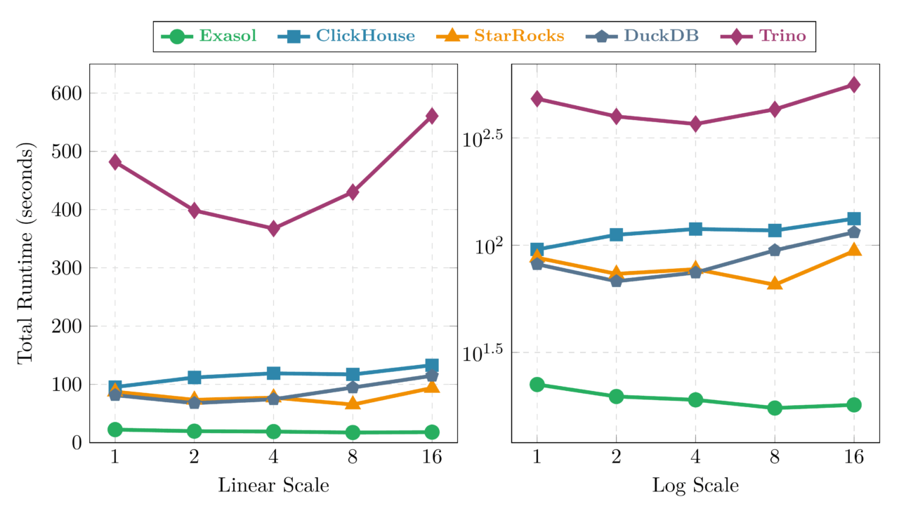
Exasol is nearly flat across the entire range: 22.4 seconds at 1 stream to 18.0 seconds at 16 streams. It actually improves slightly as concurrency grows—the optimizer finds more opportunities to share scans across concurrent queries. This is the best concurrency behavior in the test.

ClickHouse completes 18 of 22 queries at low concurrency and 17 of 22 at 8+ streams (Q05, Q09, Q18, Q21 always fail due to JOIN memory limits; Q08 also fails at higher concurrency). Among its successful queries, it rises from 95.5 to 132.9 seconds—a 1.39× ratio that nearly matches DuckDB’s degradation. Despite strong absolute performance, concurrency scaling is a weakness: per-query memory limits leave less headroom when competing for resources.

StarRocks shows a U-shaped curve: improving from 87.4s to a sweet spot of 65.4s at 8 streams, then degrading to 93.9s at 16. The FE/BE architecture benefits from moderate parallelism but shows coordination overhead at high concurrency.

DuckDB is the surprise. It degrades from 81.5 seconds at 1 stream to 114.8 seconds at 16—a 41% increase despite proportional hardware. This is the single-process architecture showing its limits: DuckDB runs all streams within one process, and at 16 concurrent query sets, internal scheduling contention outweighs the additional CPU.

Trino mirrors the U-shape: a sweet spot at 4 streams (367.5s) before JVM contention pushes it to 560.7s at 16 streams.

3.2 Throughput and Efficiency at Peak Concurrency

At 16 concurrent streams on a 64-vCPU machine, the absolute throughput gap is stark:

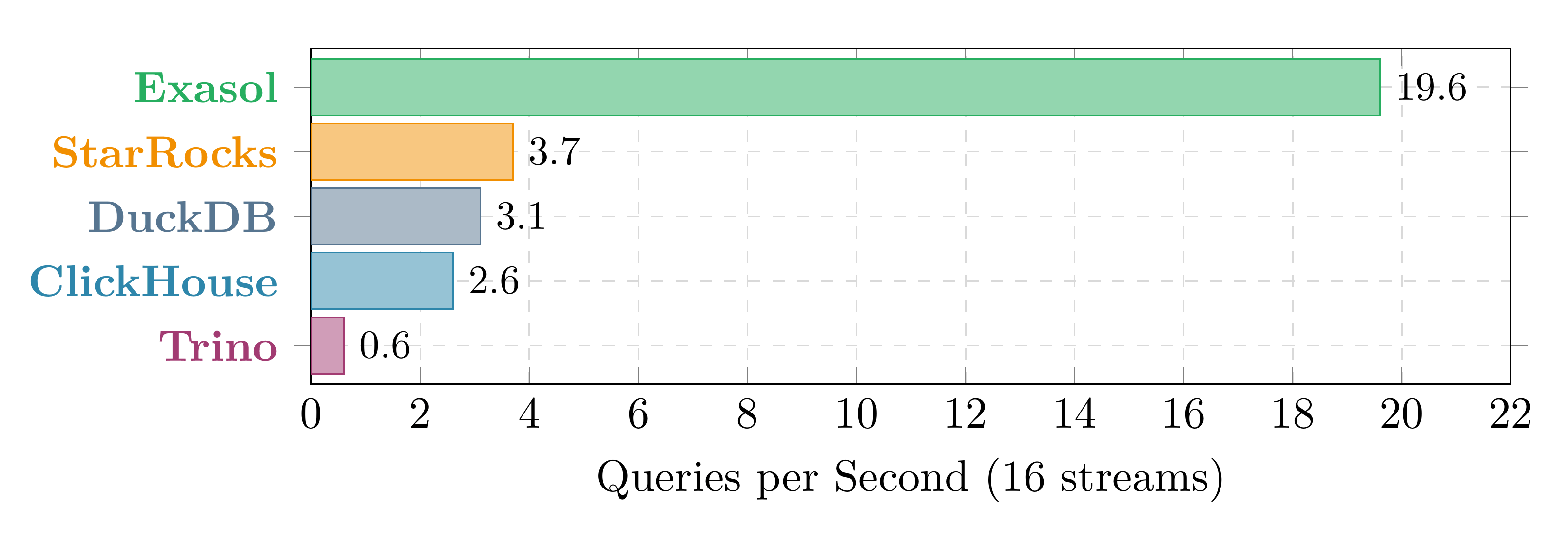
Exasol at 19.6 QPS processes 5× more queries per second than the next system.

But absolute throughput conflates engine speed with scaling behavior. A more hardware-independent metric is the scaling efficiency ratio: total runtime at 16 streams divided by total runtime at 1 stream. Ideal = 1.0× (flat). Below 1.0 = improves under load. Above 1.0 = degrades.

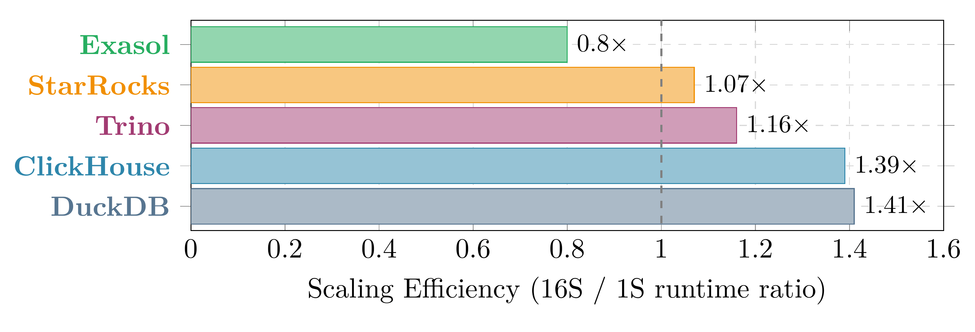
This chart is hardware-independent and directly answers: “does per-query time stay constant under concurrent load?” Exasol at 0.80× is the only system that improves. StarRocks (1.07×) and Trino (1.16×) show mild overhead. ClickHouse at 1.39× and DuckDB at 1.41× show nearly identical degradation—different architectures, same concurrency weakness.

4. Data Volume — “Can Your Database Handle More Data?”

This is the most forgiving dimension. Data grows from TPC-H SF25 (25 GB raw) to SF50 to SF100, and hardware doubles at each step: 4 → 8 → 16 vCPU, 31 → 62 → 124 GB RAM. One node, 4 concurrent streams throughout. Ideal: flat line.

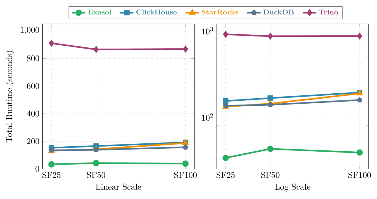
The good news: most modern analytical databases handle data growth well when given proportional resources. Exasol actually improves from SF50 to SF100 (42.8 → 38.8s, a 0.91× ratio)—the larger dataset appears to give the optimizer more parallelism opportunities. Trino achieves near-perfect scaling at 1.00×.

DuckDB (1.13×) and ClickHouse (1.16×) both stay within reasonable bounds. The SF25 → SF50 transition shows overhead for most systems—Exasol at 1.27×, StarRocks at 1.09×—which suggests the SF25 configuration benefits from data fitting more comfortably in cache.

StarRocks is the outlier at the top end: a 31% slowdown from SF50 to SF100 (142.9 → 187.8s). Something in its query execution does not scale linearly with data volume even when resources double.

Trino shows an interesting pattern: it actually improves from SF25 to SF50 (910.5 → 865.6s). JVM warmup costs are amortized better at larger data sizes, a pattern that stabilizes by SF100.

5. Nodes — “Can Your Database Handle More Machines?”

This is the hardest dimension. Total compute is fixed at 128 GB and 16 vCPU, split across 1 to 8 nodes. Going distributed introduces network latency, data shuffling, and query coordination—but there are no extra resources to compensate. Any slowdown is pure overhead. Ideal: flat line. DuckDB does not participate here because it is an embedded, single-process database.

5.1 Distribution Overhead: 1 → 8 Nodes at Constant Total Resources

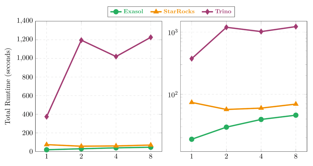
Three distinct patterns emerge:

StarRocks: the surprise. It actually improves when going distributed: 74.0s at 1 node → 57.0s at 2 nodes (0.77×), staying low at 59.9s through 4 nodes. At 8 nodes (69.5s), it returns close to the 1-node baseline—the sweet spot is 2–4 nodes where the FE/BE architecture distributes work most efficiently.

Exasol: fastest everywhere, with measurable distribution cost. At every node count—1, 2, 4, 8—Exasol posts the fastest absolute time (18.9s down to 46.1s at 8N). Distribution adds a per-doubling overhead of 1.35× (geometric mean), which is moderate for an in-memory architecture that relies on large contiguous memory pools. The cost comes from global index lookups for JOIN operations when data is split across nodes, but the absolute speed advantage over all other systems remains clear even at 8 nodes.

Trino: distribution overhead. Going from 1 to 2 nodes costs 3.19× (374.3 → 1195.9s)—the largest overhead in the benchmark, driven by inter-JVM serialization when splitting from one process to two. Adding more nodes improves things: 4 nodes (1020.2s, 2.73×) is the sweet spot, with 8 nodes (1226.7s, 3.28×) showing slight regression. The pattern: going distributed has a fixed JVM cost that amortizes only partially with more nodes.

Why ClickHouse is not on this chart. ClickHouse runtime totals are sums over different query subsets at each node count—as per-shard memory shrinks, more queries fail. Plotting 18-query totals against 8-query totals would be misleading. Its story is better told through completeness:

5.2 The ClickHouse Completeness Problem

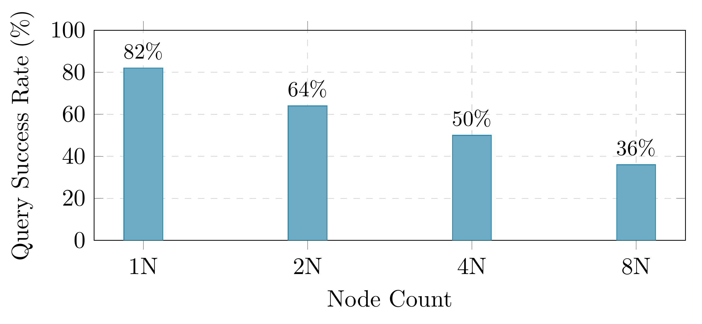
At 8 nodes, ClickHouse succeeds on only 36% of queries (8 of 22). The progression is monotonic: 82% → 64% → 50% → 36% as nodes go from 1 to 8. The root cause is per-shard memory limits: ClickHouse distributes queries across shards, and each shard receives a fraction of total memory. JOIN operations—especially FillingRightJoinSide—require hash tables that exceed these per-shard limits.

This is not a universal ClickHouse problem. For aggregation-only and filter-heavy workloads (the bread and butter of log analytics), ClickHouse scales well. TPC-H, with its multi-table JOINs, specifically stresses this weakness. A fair assessment: ClickHouse is not designed for this type of workload at scale.

For reference, Exasol, StarRocks, and Trino maintain 100% query completion across all node configurations. DuckDB achieves 100% on its single-node tests.

6. The Scalability Report Card

After 12 configurations and thousands of query runs, here is how each system behaves across all three dimensions:

System	Data1	Concurrency2	Nodes3	Reliability
Exasol	0.91×	0.80×	1.35×	100%
DuckDB	1.13×	1.41×	N/A	100%
ClickHouse	1.16×	1.39×	36% success4	36–82%
StarRocks	1.31×	1.07×	0.98×	100%
Trino	1.00×	1.16×	1.49×	100%

6.1 System Profiles

Exasol wins the most dimensions but distribution comes at a clear cost. The 1.35× per-doubling overhead means going multi-node is not free—Exasol’s in-memory architecture relies on large contiguous memory pools that lose efficiency when split across nodes. Its strongest showing is concurrency scaling, where the 0.80× ratio at 16 streams (runtime improves under load) is genuinely unusual among the systems tested. Fastest absolute time in every single configuration.

DuckDB breaks its linear scaling streak at concurrency—exposing its architectural limit. A 41% degradation at 16 streams with proportional hardware shows that the single-process design creates scheduling bottlenecks under concurrent load. For data scaling it remains solid (1.13×), and 100% reliability with zero operational complexity still makes it attractive where operational simplicity outweighs raw performance.

ClickHouse delivers competitive absolute performance but shows clear concurrency degradation: 1.39× from 1 to 16 streams, nearly matching DuckDB. Its main weakness remains distributed reliability: from 82% query success at 1 node to 36% at 8 nodes. For workloads that match its strengths—time-series, logs, aggregation-heavy queries without large JOINs—these failures never arise.

StarRocks produced the biggest surprise of the benchmark. It is the only system that improves with distribution (0.77× at 2 nodes), holding through 4 nodes before returning to baseline at 8. The FE/BE architecture handles distribution well when per-node memory is adequate. The trade-off: worst data scaling (1.31× SF50→SF100) and a U-shaped concurrency curve that degrades at 16 streams.

Trino achieves perfect data scaling (1.00×) and 100% reliability everywhere. Its weakness is absolute speed (slowest in every configuration) and significant distribution overhead: 3.19× at 2 nodes from inter-JVM serialization. Going to 4+ nodes improves scaling, but never reaches the 1-node baseline.

7. What This Means for Your Architecture

No system wins every scenario, and the right choice depends on what you are optimizing for:

• High-concurrency analytics (dashboards, many users): Exasol’s flat-to-improving concurrency curve means it gets relatively better as concurrent load increases. If concurrency is your bottleneck, this is the strongest result in the test.
• Single-machine, low-concurrency: DuckDB requires no server, no cluster management, and delivers solid data scaling. But test under your expected concurrency level first—16 concurrent streams showed 41% degradation even with proportional hardware.
• Log analytics and time-series: ClickHouse’s column-oriented engine excels at aggregation and filter workloads. Avoid complex multi-table JOINs at scale, and test under concurrent load—concurrency scaling showed 39% degradation.
• Data lake federation: Trino queries data where it lives. Absolute speed is not its selling point—flexibility is. Avoid 2-node clusters; if going distributed, use 4+ nodes where JVM overhead amortizes.
• Distributed analytics: StarRocks showed the best distribution behavior in the test—it improved 23% going from 1 to 2 nodes, with the sweet spot at 2–4 nodes. If your workload requires multi-node deployment, StarRocks handles the transition better than any other system tested.

Versions matter. These results are for specific releases tested in February 2026. ClickHouse’s memory management, StarRocks’s distributed query planning, and Trino’s JVM tuning all evolve between releases. If you see results from a newer version that contradict these findings, the software likely improved—which is the point of publishing this data.

8. How to Run Your Own Scalability Tests

Every experiment in this post was orchestrated by Benchkit, an open-source database benchmark framework. Benchkit automates the full pipeline—infrastructure provisioning on AWS, database installation and tuning, data generation and loading, benchmark execution with warmup and randomized query order, and result collection—so that an entire experiment is defined by a single YAML configuration file. The same tooling that produced these results is available in the repository; the benchkit commands in the reproduction block below are the exact interface used to run every data point published here.

All benchmark configurations are in the repository:

public/scalability/
  series_1_nodes/     # nodes_01, nodes_02, nodes_04, nodes_08
  series_2_sf/        # sf_025, sf_050, sf_100
  series_3_streams/   # streams_01, streams_02, streams_04, streams_08, streams_16

Raw result data (per-query runs.csv for every experiment):

public/scalability/reports/
  series_1_nodes/nodes_{01,02,04,08}/attachments/runs.csv
  series_2_sf/sf_{025,050,100}/attachments/runs.csv
  series_3_streams/streams_{01,02,04,08,16}/attachments/runs.csv

To reproduce a single experiment (requires AWS credentials and the Benchkit framework):

pip install benchkit

benchkit check  -c public/scalability/series_1_nodes/nodes_04.yaml
benchkit infra  apply -c public/scalability/series_1_nodes/nodes_04.yaml
benchkit setup  -c public/scalability/series_1_nodes/nodes_04.yaml
benchkit load   -c public/scalability/series_1_nodes/nodes_04.yaml
benchkit run    -c public/scalability/series_1_nodes/nodes_04.yaml
benchkit infra  destroy -c public/scalability/series_1_nodes/nodes_04.yaml

If you find something wrong—a data point that does not match the CSV, a chart that misrepresents the methodology, or a conclusion that does not follow from the numbers—open an issue. Reproducibility means being willing to be corrected.